Learning Which Computations to Trust:
Audited Solver Choice, Fallible Verification, and Drift
AI-assisted research draft
13 November 2026 — isolated research revision 3
Classification: Technical methods note. Standard decision and concentration tools applied to a declared solver interface; no new general metareasoning principle or priority claim.
Abstract
An agent can use a model of its computations to choose a solver, verify its output, or invoke an exact fallback. We give a finite operational contract in which approximate solvers generate candidate witnesses, a trusted checker reveals correctness at a cost, and an exact solver repairs a failed candidate. A five-action deployment menu has an explicit cost frontier. Independent audited training gives a simultaneous calibration guarantee and a finite-sample excess-cost bound; a margin condition is required to compare certified policies with a known-reliability oracle. A finite-horizon Bayesian recursion distinguishes verification for the current answer from verification that also improves future solver choice. For independent errors with slowly changing means, a sliding audit window has an explicit sampling-error plus drift-bias bound. Executable partial-constraint solvers and exact finite-state calculations illustrate these results, including cases where additional computation is redundant or current verification is costly but future learning makes it worthwhile. An extended contract prices controller overhead, derives residual risk for fallible checking, and gives a sparse scheduled noisy-audit bound with a warmup bill. A finite hidden-state recursion handles noisy learning and switching costs. Direct gold-label calibration also bounds invalid acceptance without a known checker channel. A frozen public SAT study and a disclosed larger-instance amendment measure complete pipeline and setup costs. Risk-constrained selection chooses the fixed exact solver, and a mature exact baseline further strengthens the negative result. The work is a limited synthesis of established metareasoning, algorithm selection, and risk calibration. It establishes neither universal architectural superiority nor subjective introspection.
1 The computational question and its antecedents
Metacognitive control is useful only if a model of computation changes which computation is performed or how its output is used. A verbal confidence label without consequences is not the object of study. Here, the controller learns how often particular algorithms produce invalid candidate witnesses on a declared task distribution, and uses that knowledge to allocate verification and fallback computation.
Hay, Russell, Tolpin, and Shimony formalize computation selection as a metalevel decision problem with explicit computational outcomes and costs [6, Definitions 1–3 and Theorems 4–5]. Algorithm portfolios already learn which solver to use and how to schedule alternatives; Kadioglu and colleagues provide a concrete selection/scheduling framework and matched SAT benchmarks [10, Sections 2–4]. Neither choosing an algorithm from experience nor the expected value of computation is introduced here.
The nearest B-Theory note, When Checking Takes Time, version 1.0 of 9 November 2026, gives an exact two-probe stopping example with a changing external mechanism and known noise [2]. Finite Noisy Audits with Learned Baselines, version 1.0, already prices observations and separates learned baselines from audit evidence [3]. The change here is the provenance of the outcome: it is produced by an executed candidate-generation algorithm, and correctness is supplied only by a paid checker. The mathematical reduction still uses ordinary statistics. This provenance supports an operational interpretation as computation control; it does not make a familiar concentration inequality a new metacognition theorem.
The results below should be read as a methods note and a reproducible starting model. Their strongest contribution to the portfolio is a precise distinction between current answer quality, the cost of verification, and information about future computation quality. General policies that combine arbitrary solver traces, nonstationarity, and scarce verification remain unresolved.
2 Operational contract
Tasks arrive in observed regimes . In the stationary part, independent instances are drawn from an unknown fixed distribution . Each instance has a nonempty finite witness set
Two supplied randomized algorithms read , execute their prescribed partial computation, and output a candidate . The complete checker computes whether that candidate is valid. An exact algorithm returns a valid witness. Algorithms, checker semantics, and action costs are common knowledge; their population error rates are initially unknown. Solver coins are fresh across tasks. Errors from different solvers on the same task may be dependent.Running solver costs , checking a returned candidate costs , and invoking the exact solver costs . Costs are normalized task-loss units, not measured seconds. An invalid terminal witness incurs additional loss one. An exact fallback always terminates within the stated task deadline. The instance and target do not change during computation. No unpriced evaluator reveals whether an unverified answer was correct.
For the first result the controller has five permitted deployment policies:
| Policy | Executed operations | Expected task loss |
|---|---|---|
| run , return candidate | ||
| run , check, use only if invalid | ||
| run exact solver |
There are two policies of each indexed type. Verified policies have zero terminal error under the trusted-checker and exact-fallback assumptions. Their running cost varies with candidate validity. The menu excludes inspecting extra solver traces, combining candidates, or using input features beyond to choose the menu entry. Those are meaningful extensions rather than secretly available privileges.
This model has genuine computational acts: the candidate is computed from the task instance, the verifier executes a correctness test, and the fallback constructs a solution. Nevertheless, retaining only the error indicator gives a Bernoulli statistical interface. Our theorems concern that interface, not a separation from every possible algorithm on . An unrestricted compiler could encode the same choice mapping, and a different exact algorithm could have a different cost. In Sections 2–8, fixed code, controller memory, and exact real arithmetic are unpriced; later sections extend the accounting and report bounded implementation measurements. The comparisons make no asymptotic implementation claim.
4 Learning reliability from an audited training sample
For each regime, collect independent training tasks and run both solvers and the full checker on each candidate. This full-information audit costs (3) The exact fallback is not run during training. Training tasks have no additional deployment-success obligation; if they did, that cost would have to be added. Let indicate the error of solver on task in regime , and let .
Lemma 4.1 (Standard bounded-sample concentration). For independent variables in with means , their mean satisfies Identical distributions are unnecessary.
This is Hoeffding’s inequality [7, Theorem 2]. To make the dependence explicit, for a bounded variable the centered log moment-generating function has second derivative equal to a tilted variance, at most . Its value and derivative at zero vanish, so it is at most . Multiplying these bounds over independent variables, applying Markov’s inequality, and minimizing at for the average gives for either tail; add the two tails. The variance bound follows from for any law on , including the tilted law.
Put and (4) For each , let minimize over the five entries, with a fixed public tie rule.
Theorem 4.2 (Simultaneous calibration and menu regret). With probability at least over the training sample, simultaneously for all , and simultaneously for all regimes, (5) The same event supports every predeclared mixture of the regimes at deployment.
Proof. Apply Lemma 4.1 to each of the empirical error rates. A union bound gives failure probability at most . Independence between the two solvers on the same task is not used. On the good event, every menu loss changes by at most , because its dependence on a single error rate has slope zero, one, or . If minimizes true loss, then
Average these simultaneous inequalities with any fixed nonnegative regime weights summing to one. ◻This is a finite-action empirical-risk comparison using a standard uniform bound. The known-reliability oracle is privileged and pays no calibration charge. For deployments the learner’s good-training-event expected total cost is bounded by for the chosen regime mixture. It is incorrect to omit or to describe a high-probability conditional bound as a deterministic bill. An unconditional bound adds at most per deployment, where bounds possible regret.
4.1 A certified-error constraint needs a margin
Suppose terminal error must be at most in each regime. Permit only when ; keep available. Select the cheapest estimated loss from this certified menu.
Corollary 4.3 (Risk certification with a comparator margin). On the same event, every selected policy has terminal error at most . Its loss is at most above the best of the exact/verified policies and the unverified policies satisfying .
Proof. Every admitted unverified policy has ; all other entries have zero terminal error. If , then , so that comparator is admitted. Apply the same two-error comparison as in Theorem 4.2. ◻
The loss comparison deliberately excludes an unverified oracle action exactly on the risk boundary unless it is independently certified. Uniformly matching a boundary oracle from finite data would require a stronger argument. Certification is a property conditional on the training event and the assumed unchanged deployment distribution, not a guarantee that a particular emitted witness is correct.
5 Verification can have value for future tasks
An alternative contract learns during deployment. For one regime, suppose the error rates are independent latent variables . Conditional on the rates, solver errors on successive tasks are independent; unverified candidates supply no correctness feedback. A verified error increments and a verified success increments . No update follows an exact-only action. Let , , and denote failure and success updates.
Proposition 5.1 (Standard finite-horizon metalevel dynamic program). With tasks left, the optimum Bayes total cost within this online menu is and (6)
Proof. The beta posterior follows by multiplying its density by after a verified failure or by after a success. Predictive failure probability is . Condition on the first menu choice and, for verification, its two possible outcomes. The immediate expected costs are exactly those of Proposition 3.1. Posterior parameters contain all retained information relevant to future task errors in this stipulated exchangeable model. Backward induction over the finite horizon proves the recurrence and permits a deterministic minimizer at each state. ◻
This recursion is not a new form of rational metareasoning; it makes one feedback assumption explicit. If unverified answers later receive trustworthy labels, the second line must also branch and learn. If errors depend on retained solver state or correlated task families, the beta counts are not sufficient.
The reproducible example takes , an unknown solver-1 error with prior , and a known solver-2 error . At the initial mean, unverified solver 1 costs and verified solver 1 costs . Thus checking is worse for the isolated current task. The supplied exact rational recursion evaluates horizons and records how future information changes the initial choice. This is a Bayes planning example under a supplied prior, not an empirical claim about general reasoning quality.
| Horizon | Optimal expected cost | First action | Always cost |
|---|---|---|---|
| 1 | |||
| 2 | |||
| 5 | |||
| 10 | |||
| 20 |
6 Slow drift and stale solver calibration
Now fix a regime and allow independent error indicators with changing means . Assume the deterministic rate constraint
For this extension, each task first commits to and completes one deployment-menu action using only earlier audit labels. A separate audit then reruns both solvers with fresh private coins on the saved current instance and checks both new candidates. These correctness labels are disclosed only after the terminal deployment answer, so they cannot repair a nominally unverified answer on that task. Both reruns and both checks are charged, even when they duplicate production work: the fixed additional per-task audit cost is The cost for choosing entry is therefore . Comparators in the drift result use this same audit protocol. No computational reuse or unpriced current feedback is assumed. Before task , estimate from the preceding audits,Theorem 6.1 (A fixed-window drift bound; standard concentration specialization). For a predeclared horizon of at most evaluated tasks and window , with probability at least , simultaneously for the two solvers and all evaluated times, (7) Plug-in menu selection then has current expected deployment-menu excess loss at most at every such time on this event. Adding the common audit charge to both comparator costs preserves that difference; it does not remove the audit expenditure from total cost.
Proof. The mean of the window estimator is the average of its possibly unequal Bernoulli means. Lemma 4.1, applied at each fixed window, and a union bound over at most windows bound deviations from those averages by the first term. Overlap between windows does not affect the union bound. The deterministic drift condition gives
Combine the two inequalities and repeat the loss comparison from Theorem 4.2. ◻The theorem is not valid for an adaptively chosen window without accounting for that selection, nor does it infer from the same data. Its formula quantifies the tension between a long window’s reduced sampling error and increased staleness. Minimizing the two variable terms over real gives the usual scale when , before integer and horizon constraints. No minimax optimality is claimed. Section 10 treats deterministic sparse noisy audits; adaptive sparse verification, abrupt changes, and input-dependent nonstationarity remain unresolved.
7 Executed finite constraint-solving study
The illustration uses witnesses . An instance contains two membership predicates with a nonempty intersection. Solver enumerates candidates satisfying and chooses one uniformly; it defers the other constraint. The full checker evaluates both. The exact fallback scans candidates and returns the first satisfying both. A uniformly rotated labeling creates sixteen instances per regime. Every solver, verifier, and comparator receives the same instance; no hidden task label is exposed to one controller alone.
The three regime families have candidate-set sizes and intersection sizes
| Regime | Oracle menu choice | ||||
|---|---|---|---|---|---|
| A | 10 | 15 | 9 | , loss | |
| B | 15 | 10 | 9 | , loss | |
| D | 5 | 5 | 3 | , loss |
The error formula is . The complete task sets, rotations, and solver code are supplied. Enumeration checks 48 task instances and 96 solver error laws. A separate seeded execution runs each solver 20,000 times per regime, totaling 120,000 trials, as an implementation check. This is synthetic computation, not a benchmark showing a practical speedup.
The figure’s learning curves are finite sums over the two binomial training error counts, with . Independent solver seeds and the constant regime-specific error rates justify the product of the two count laws in this example; the general guarantee does not require within-task independence. The sums are evaluated in floating point and saved with the known-rate comparator. They describe expected deployment cost; the separate training cost is recorded rather than hidden in the plot.
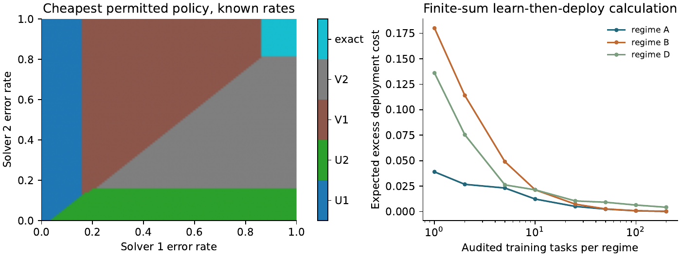
The supplied costs deliberately isolate the decision problem. On such small explicit sets, another implementation could directly compute the intersection and cheaply solve every task. Therefore the illustration establishes a checkable solver-feedback contract, not a computational advantage over all programs. Real algorithm portfolios must measure feature extraction, checker, solver, switching, and controller overhead on a suitable task distribution.
8 Counterexamples and limits of inference
Biased verification.
Let half the tasks be easy with solver error zero and half hard with error . Auditing only easy tasks estimates error zero even with unlimited data, while the overall error is . Theorem 4.2 does not apply: training is no longer representative. Adaptive auditing needs an explicit missing-feedback correction, randomized sampling design, or a valid conditional model.
Re-running a deterministic computation.
If a solver sees the same input and retains the same seed or deterministic state, it returns the same candidate. Repeating it without a new check adds no information about validity and consumes positive cost. Multiplying its marginal error rates as if repetitions were independent creates fictitious confidence. New independent seeds alone also do not imply conditional independence of failure for arbitrary shared task difficulty.
Marginal calibration is not introspective certainty.
A regime-average error rate can be accurate while errors are concentrated on one narrow family of inputs. These results calibrate population rates, not confidence for every answer. Instance-level reliability needs a richer observation model and held-out conditional validation.
A drifting world during deliberation.
The task instance remains fixed until a final witness is returned. If the target changes while a solver runs, runtime changes the target distribution and verification can become stale. A common deadline or a clearly indexed target is required before comparing policies; the earlier two-probe B-Theory note studies a different timing contract. Its conclusions should not be imported without a new derivation.
The checker is a trusted resource.
If can be wrong, verified policies no longer have zero terminal error. Shared bugs between candidate generation and checking can defeat repeated agreement. A genuinely uncertain checker requires a second reliability model, identifiable references, and a cost for validating it. D03’s evidence-validity problem then becomes relevant; the later known-channel extension does not identify an unknown checker or resolve an infinite regress of verification.
9 Fallible checking and controller costs
Sections 2–8 retain the trusted-checker contract. We now change it explicitly. These additions are finite-model specializations, not a claim that realistic verification or general metareasoning has been solved. Let denote an invalid candidate and denote rejection by a fallible checker. Assume known conditional rates
These rates must hold for the deployed solver, candidate population, regime and time, including each latent state below. Accuracy on an unrelated checker test set does not suffice. A rejection invokes the exact fallback; an acceptance returns the candidate. Call this policy , reserving for the earlier trusted checker. Exact fallback remains an assumption.Let be fixed deterministic controller charges in the same loss units. They can include dispatch, feature extraction, memory updates and amortized offline construction, if billed once. Memory, time and energy need declared conversions or separate constraints; arbitrary resource units cannot be added.
Proposition 9.1 (Fallible-check frontier). Writing , the action losses and terminal errors are
| Action | Expected loss | Terminal error |
|---|---|---|
Their minimum is the five-entry menu optimum. Checked action strictly improves on exactly when (8)
Proof. The joint masses for are . Fallback has probability ; invalid acceptance has probability . Summation and subtraction give the claims; randomization remains a convex combination. ◻
Equal controller charges and recover the original frontier. False rejection pays for unnecessary fallback; false acceptance leaves residual error. A checker with always accepts and provides neither repair nor information. Repeating an identical shared bug does not fix it.
9.1 Identification and certified decisions
Rejection frequencies alone do not identify both solver and checker reliability. The models and both give , but checked terminal risks are zero and . Even infinite independent labels with this identical law do not distinguish the models through this interface. Known noise correction and identifying the noise matrix are different problems [11]. Gold references or additional identifiable structure must be supplied and priced.
Suppose known channels and clipped estimates satisfy . Put
For an error limit , admit only when , only when , and always admit . All admitted actions are safe on the confidence event. Write . A comparator whose true risk is at most is admitted because . Zero-slope risks need no margin.If estimated controller charges have uniform error at most and an implementation returns a certified action within of the smallest estimated certified-menu loss, its excess over the best margin-admitted comparator is at most (9) Every estimated action loss differs from truth by at most ; adding this error on both sides of the approximate minimization proves the statement. This does not supply runtime confidence bounds or a certified numerical optimizer for free. With switching costs, a one-step comparison is from the same previous-action state, not against a globally optimal switching sequence.
Estimated cannot be treated as exact here. Given an independently justified simultaneous confidence set for , the rule guarantees safety whenever covers truth. Constructing, computing and paying for that set remains part of the calibration experiment; no learned-checker experiment is claimed.
10 Sparse scheduled noisy audits under drift
In this contract are deterministic means with . Current deployment outcomes must have these laws conditional on earlier disclosed audit history; independent tasks and fresh coins suffice. Each scheduled audit separately reruns both solvers and noisy checks after the production answer. Its charge is , including audit processing. Assume known time-invariant channels with , independent audit labels across tasks for each solver, and deterministic audit times fixed before observing labels. Within-task dependence between solvers is permitted. This protocol uses only audit-copy labels, deliberately ignoring production checker feedback.
Before evaluated task , the last audits have times . Define
The window and horizon of at most evaluated tasks are predeclared. Purchase sufficient prehistory audits or begin the guarantee after warmup.Theorem 10.1 (Noise and audit-age bound). For , with probability at least , simultaneously over two solvers and at most evaluated tasks, (10) Plug-in menu selection has conditional expected deployment-loss excess at most . Approximation and certification use the modified rules above.
Proof. Each label mean is . Hoeffding and a union bound control every window’s deviation from its own mean by the square-root term before inversion. Inversion divides this fluctuation by and maps the expected rejection average to the average of past values. Its distance to current is at most . Projection cannot increase distance to and the distance is at most one. Apply the loss slopes and conditional deployment-law assumption. ◻
The drift term is not divided by . Known negative is also invertible, with in the sampling denominator. At , labels are uninformative about . Checker drift invalidates this fixed-channel derivation.
With period , the latest audit age is and . For common and , balancing the variable terms gives
This minimizes a bound, not minimax regret. Choosing deterministically from design parameters is allowed; adapting them to labels needs another proof.For common learner-only controller charge , a known-rate oracle paying neither controller nor audits, warmup audits and at most deployment audits, the good-event difference of predictable expected total losses is bounded by (11) Here base menu losses exclude that separately charged common ; includes offline design and channel calibration. The statement concerns expected stage losses on a confidence event, not realized bills, a fair-resource oracle, or a runtime deadline guarantee. Unconditional expectation needs a bounded bad-event remainder. Only costs actually shared by a comparator cancel.
The design calculation uses and optimizes separately for . With known channels and , period , window gives radius and upper bound per deployment; period , window gives . The bound is loose and certifies no practical improvement. Warmup costs , takes time steps, and requires the drift law over that prehistory. This is a deterministic bound-design calculation, not a simulated optimal audit policy.
11 Bayesian noisy feedback and hidden drift
This is a separate stochastic contract. A finite hidden state has known transition matrix applied after each task. Conditional on the state, fresh error probabilities are and the checker channel is stable. The belief precedes computation. In the abstract controller interface only a checked outcome supplies learning: candidate identity, input features, runtime, fallback witness and realized error penalties reveal no further information. An implementation exposing such signals needs a changed observation kernel.
Write , and . Bayes’ rule gives
A zero-probability branch contributes zero and needs no posterior definition. Let be the previous menu entry, a switching charge (initially zero), and the noisy-check table’s immediate loss using posterior means.Proposition 11.1 (Finite-horizon belief recursion). With , the optimum within this interface is
Proof. Condition on the first action and its available observation. Update the current belief before applying the state transition. Without observations the prediction is . Remembering accounts for switching costs. Backward induction gives optimality on the finite history tree. A finite hidden-state space does not imply a finite belief space for an unbounded horizon. ◻
Noisy rejection cannot increment the original beta failure count: its likelihood is , not . Multiplying a beta density generally produces a mixture. With , either label leaves the posterior unchanged; the code tests this counterexample. This Bayesian model is not automatically covered by Theorem 10.1; posterior jumps do not supply its deterministic-mean assumptions.
Exact examples use solver-1 rates with equal initial weights, known solver-2 rate , , , checker prices , symmetric state-flip probabilities , and switch charges . These priors differ from the original beta example, so differences cannot be attributed to noise alone. Eighteen exact cases at horizons record fractions, first actions, state counts and planning times. Policy-tree evaluation checks achieved values using the selected Bellman policy; it is not another optimality proof. A separate specialist implementation independently reconstructs the three displayed horizon-eight optima by exact alpha-vector policy-tree enumeration with rational lower-envelope pruning, without reusing the posterior recursion.
| Horizon | Checker price | Flip probability | Optimum loss | First action |
|---|---|---|---|---|
| 8 | .06 | 0 | .960000000 | |
| 8 | .02 | 0 | .959498712 | |
| 8 | .02 | .02 | .960000000 |
These displayed rows have zero switching charge; the full table includes the positive-charge cases. The middle value is exactly . Its first checked action costs versus unverified. Future information gives a small net gain, while hidden drift removes it in the displayed comparison. No universal horizon threshold or robustness claim follows.
12 Audit evidence, measured costs, and research limits
All five regenerated original data files match their delivered bytes. The earlier review closure’s source and code hashes match the delivered artifacts. A separate new specialist implementation reproduces all five original rational Bayesian values and checks 27,951 rational noisy-channel cases. The new author implementation separately checks 14,641 joint-event cases. Printed proofs support general claims; finite checks support implementation consistency. New reviews are internal AI reviews, not human peer review.
The original five-task advantage over always is
An additional uniform per-task controller charge relative to that fixed baseline erases this particular gain at . A one-time additional charge has break-even . These statements concern the specified policy comparison, not every possible policy. A common charge can leave action rankings unchanged yet erase an advantage over a cheaper fixed implementation.The local timing experiment uses all 48 prepared original instances, three warmup batches and 21 measured batches of 4,800 calls, with shuffled operation order and raw nanosecond records. It measures partial candidate generation, checking, scan-based exact solving, direct exact intersection, floating menu calculation and a compiled lookup. Direct intersection is faster in this recorded environment than either candidate generation or floating menu calculation. Thus the tiny tasks support no portfolio speedup claim. They do not turn synthetic loss prices into realistic costs. Dispersion across batches is not a confidence interval across workloads or machines. Cold input construction and hard deadlines are excluded. Exact rational planning times and state counts are recorded separately. Compiling a policy can save online planning but incurs construction, memory, lookup and model-obsolescence costs.
Charging selection overhead is established practice: SATzilla includes feature and presolver time and a timeout fallback [16, Sections 4.2–4.3]. Costly-feedback learning and paid multi-arm observations already appear in Tucker et al. [15], Seldin et al. [14]; current contextual work also includes observation expenditure [5]. Smooth nonstationary bandits have stronger results under different time/feedback assumptions [9]. No regret-rate transplant or priority claim is made. The increment here is an auditable repaired-output loss, known noisy-check channel, sparse scheduled-audit certificate, and exact counterexamples and implementation checks.
Revision 2 left learned-checker calibration and public-task cost validation open. Sections 13–15 address direct gold calibration and bounded public-corpus validation; adaptive biased audits, unknown abrupt drift and representative solvers under a common deadline remain substantive blockers. Gold labels and exact fallback reliability remain paid resources.
Share generic concentration and noisy-channel methods with D03/D04. D03 owns physical evidence freshness; D05 owns recurrent resource viability; D07 owns memory/coding; D10 owns a specified physical energy boundary. D08 owns solver-produced candidates, checker feedback, repair choices and controller costs. This revision makes no joint theorem about those manuscripts and edits none of them. The operational capability does not establish consciousness, subjective introspection or intrinsic superiority of explicit self-model terminology.
13 Gold-label calibration without a known checker channel
The known-channel assumption of Section 9 is avoidable when calibration pays for trusted truth. This changes the information contract: rejection-only observations still do not identify residual error. Fix solver/checker pairs and an unchanged iid task population. On calibration draw , let indicate an invalid candidate, as determined by paid gold checking, and let indicate rejection by the deployed fallible checker. Set . Arbitrary within-task dependence is allowed. Draws, including solver and checker randomness, are independent across tasks. Exact repair on rejection gives
The terminal error of is . Neither conditional checker ratios nor a lower bound on invalid-candidate prevalence is needed. Rare invalid candidates can make a conditional false-acceptance estimate unstable while the joint event remains directly estimable.Theorem 13.1 (Finite-menu joint-event calibration). Let be positive integers, and . Assume deterministic nonnegative prices, known , and exact repair, with unit terminal-error loss. Let and . From gold-audited iid tasks form empirical means of and . Admit when , admit when , and always admit the exact baseline. Suppose each action’s deterministic total price is estimated within and selection is within of the smallest estimated admitted loss. With probability at least , every admitted action has error at most , and excess expected loss is at most relative to the best action whose true uncertain risk is at most , together with the always-admitted exact baseline.
Proof. Rejection and invalid acceptance are disjoint, so and . Hoeffding’s inequality and a union bound over the variables give simultaneous absolute errors for the normalized means. Unverified loss error is at most and checked loss error at most . Upper risk bounds imply safety. For a comparator with risk at most , its estimated risk plus is at most , so it is admitted. Comparing its estimated loss with the selected one and paying the two loss-estimation errors proves the assertion. The exact baseline requires no risk margin. ◻
Here bounds each action’s total additive deterministic price error, not each constituent price separately. If is estimated, its contribution must also be covered by a uniform action-total loss-error bound; the displayed proof uses known . A separate simultaneous interval for requires concentrating variables instead, with . The theorem concerns population risk and expected loss, not correctness of each returned witness. Gold calibration costs are paid before deployment. If the checker, population or solver changes, this certificate does not automatically transfer. This is a standard finite-family risk-calibration specialization, closely aligned with Learn then Test’s uniform-risk selection result [1, Section 2.5, Proposition 7]; it is not a new general learning principle.
13.1 Variable costs and finite-horizon billing
For task-dependent exact work , expected repair expenditure is , not . On two equiprobable tasks with and , the former is and the latter . End-to-end measured action costs preserve this dependence. With a declared almost-sure bound on complete realized loss, direct bounded-loss calibration is possible; observed wall-clock maxima alone do not supply that bound. A timeout changes the answer interface and must be modelled.
Let be actual setup costs and the expected deployment saving of a fixed calibrated controller over a specified fixed baseline. Its expected total saving over further tasks is
Only a positive justified lower bound on supports a certified break-even claim. Charging common setup to both sides is appropriate only when both implementations incur it. The study below reports measured bills and empirical projections, not a wall-clock concentration theorem.14 Public SAT witnesses: calibration, full costs, and negative results
14.1 Frozen primary protocol and probability target
The primary protocol was recorded before downloading or inspecting outcomes. SATLIB’s UF20-91 corpus contains 1,000 satisfiable random 3-SAT formulas with 20 variables and 91 clauses [8]. All source files, archive hashes, split, seeds, witnesses and operation timings are retained. A fixed random split assigns 600 formulas to calibration and 400 to testing. Algorithm seeds depend on formula identity, solver and replication, independently of the split. No timeout changes binary outcomes. This supports a fixed finite-population probability statement, not an iid claim about future SAT workloads.
Proposition 14.1 (Held-out finite-population risk certificate). Let be integers with , , and . Fix binary potential outcomes for each of predeclared seeded policies. Sample calibration tasks uniformly without replacement, and observe errors for a policy. Put and define Then simultaneously for all policies, with probability at least over the split, the actual residual-error fraction on the remaining tasks is at most .
Proof. For the true total , the discrete lower-tail -value obeys . If is retained then ; exclusion occurs only in that lower-tail event. The feasible set is nonempty since . Apply a union bound across policies. Independence between policies is unnecessary. ◻
This elementary exact inversion certifies the remaining fixed seeded corpus, not fresh seeds, new formulas or drift. It allows data-dependent choice among the predeclared policies but does not transfer the iid theorem’s comparator margin or certify timing optimality. An independent integer-arithmetic implementation checks all 2,552 small-population coverage cases and the actual experiment’s bounds. For , zero observed errors gives a statistical upper bound , not zero. Structural zero error under an exactness contract is a separate claim.
14.2 Executed alternatives and accounting
The exact baseline is a pedagogical Python DPLL solver. Candidate solver solves the first 45 clauses, filling unspecified variables with false; performs at most 80 WalkSAT-style flips, with noise probability , retaining its already-computed full-formula validity flag. Neither is an industrial approximation baseline. The eight policies are , unverified , partial-check-and-repair , full-check-and-repair , and trace-aware . The partial checker samples 15 distinct clauses uniformly; reuses ’s validity flag and avoids redundant checking. Each path separately executes its actual reads, parsing, solver randomness, checker and conditional fallback. A literal-level full-clause evaluator labels outputs after deployment timing; its calibration work is charged. It shares the parser with the implementation and is not a formal independent parser proof.
Calibration selection minimizes measured seconds plus times empirical terminal error for seconds per invalid answer, subject to held-out risk upper bound . Choices are locked before test execution. This is global calibrated selection, not demonstrated per-instance adaptive control. Primary test replication zero contains 400 tasks; two further seed replications are sensitivity runs on the same tasks, not 800 new independent tasks. Timings are read/parse-inclusive; cold page-cache conditions are not imposed. Raw records provide -ms exceedance fractions; these are descriptive thresholds, not enforced deadlines.
| Policy | Invalid / 400 | Mean time (ms) | Calibration error bound |
|---|---|---|---|
| 0 | 1.103 | .0125 | |
| 400 | .390 | 1.0000 | |
| 143 | 1.360 | .4050 | |
| 149 | .975 | .4475 | |
| 88 | 1.504 | .2650 | |
| 0 | 1.267 | .0125 | |
| 0 | 1.726 | .0125 | |
| 0 | 1.704 | .0125 |
The last column is the statistical upper bound for the held-out seeded error fraction from calibration, not a confidence interval based on the displayed test errors. Exact and fully repaired policies additionally have structural zero risk under their correctness assumptions. Every constrained choice selects at all four loss scales. The unconstrained choice selects only at the smallest scale and otherwise. Thus this experiment supplies no controller advantage. Recorded setup, calibration and selection consume seconds (including seconds of pipeline work and seconds of gold labeling). At 400 deployments, fixed costs about seconds; the learner adds the setup bill and dispatch work. Larger-horizon totals replay empirical means and are explicitly projections. Network transfer, dependency installation and research development are outside this operational setup bill and documented separately.
14.4 Exploratory mature-solver and size-transfer amendment
After the primary results, a disclosed amendment adds pycosat 0.6.6’s PicoSAT backend [12] and 100 UF50-218 formulas, selected by a fixed filename-hash rule from SATLIB’s 1,000-formula corpus. No controller parameters are retuned. PicoSAT is a mature exact baseline, not claimed to be current state of the art. It and a fresh reference are interleaved on all 400 primary test tasks; all nine policies run on the 100 larger formulas. This amendment is exploratory, and the primary certificate is not transferred.
| Corpus | Policy | Invalid / tasks | Mean time (ms) |
|---|---|---|---|
| 20 variables | PicoSAT | 0 / 400 | .282 |
| 20 variables | fresh | 0 / 400 | 1.282 |
| 50 variables | PicoSAT | 0 / 100 | .783 |
| 50 variables | 0 / 100 | 26.126 | |
| 50 variables | 100 / 100 | .855 | |
| 50 variables | 87 / 100 | 5.639 | |
| 50 variables | 18 / 100 | 22.670 | |
| 50 variables | 65 / 100 | 11.064 | |
| 50 variables | 0 / 100 | 28.080 |
The exact mature baseline is faster and error-free in these recorded comparisons, including against the unverified candidates. Full verification and trace-aware repair do not produce a measured advantage. Partial-checker outcomes change sharply with task size; neither constant channel parameters nor certified drift robustness follow. One machine, small satisfiable random formulas, a limited solver family and no hard deadlines preclude industrial or general efficacy claims. Installation/compiler details, imported binary hash, raw results and selected-file manifest are retained.
15 Contribution boundaries and human-review questions
Learn then Test already permits arbitrary selection from uniformly risk-controlled parameter families and multiple risk constraints [1, Sections 2.4–2.5]. ASlib standardizes algorithm-selection scenarios, instance features and their costs [4, Section 2]; SATzilla already prices portfolio overhead [16]. Recent SHIP work calibrates complete verifier-guided release policies against a separate target judge, with a prespecified grid and explicit calibration expenditure [17, Sections 3.3–3.4, Proposition 2]. Its selective, judge-relative image loss differs from D08’s unconditional binary invalid-witness risk after exact repair, but the policy-level calibration principle overlaps directly. Its experiments were not reproduced here. ORACLE already combines model routing, task-dependent verifier choice and asynchronous feedback [13, Sections 4.1–4.2]. Its reported cost excludes classification, verification and routing calls [13, Section 5.1]; D08 prices a different, complete pipeline. This accounting distinction is not a head-to-head performance result or a criticism under ORACLE’s declared scope. The joint-event certificate, hypergeometric inversion, conditional-cost identity and setup break-even identity here are applications of established tools. The defensible contribution is their explicit integration with candidate generation, imperfect checking and exact repair, together with preserved negative cases and executable evidence. No claim of being the first such integration is established.
The public-corpus study improves on toy timing evidence by checking 14,800 primary/diagnostic records and adding 1,700 exploratory rows. Independent AI review reconstructs truth labels, seeded checks, exact calibration bounds and billing; six primary formulas also receive complete truth-table enumeration. Finite computation is implementation evidence, not a proof of general solver correctness. All review is simulated/internal AI review; no external human peer review has occurred.
Gold labels resolve rejection-only nonidentifiability in the declared stationary contract, but do not solve calibration without trusted labels, adaptive audit bias, unknown abrupt drift, informative solver traces beyond the stated interface, industrial deadlines or deployment under distribution shift. A useful next study needs a task family where a strong fixed solver is actually expensive, an independently justified checker, a declared loss scale and complete overhead pricing. The concrete human-review questions are whether this limited synthesis merits a methods note, whether the finite-corpus safety target is useful, and whether a proposed next workload can test a plausible advantage before expensive deployment. Portfolio ownership remains as stated in Section 12; related manuscripts are contextual sources, not shared edited artifacts.
References
- Anastasios N. Angelopoulos, Stephen Bates, Emmanuel J. Candès, Michael I. Jordan, and Lihua Lei. Learn then test: Calibrating predictive algorithms to achieve risk control. The Annals of Applied Statistics, 19(2), 2025. doi: 10.1214/24-AOAS1998. URL https://arxiv.org/abs/2110.01052. Uniform-risk selection: Section 2.5, Proposition 7 in arXiv v5; multiple risks: Section 2.4.
- B-Theory research programme. When checking takes time: An exact two-probe stopping frontier, 2026. URL https://www.b-theory.com/manuscripts-html/when-checking-takes-time/. Technical addendum, version 1.0, 9 November 2026. No individual author line in supplied source.
- B-Theory research programme. Finite noisy audits with learned baselines: Exact risk, interface-dependent memory, and a matched compiled controller, 2026. URL https://www.b-theory.com/manuscripts-html/finite-noisy-audits/. Technical addendum, version 1.0, 9 November 2026. No individual author line in supplied source.
- Bernd Bischl, Pascal Kerschke, Lars Kotthoff, Marius Lindauer, Yuri Malitsky, Alexandre Frechette, Holger Hoos, Frank Hutter, Kevin Leyton-Brown, Kevin Tierney, and Joaquin Vanschoren. Aslib: A benchmark library for algorithm selection. Artificial Intelligence, 237:41–58, 2016. doi: 10.1016/j.artint.2016.04.003. URL https://arxiv.org/abs/1506.02465.
- Xueping Gong and Jiheng Zhang. The cost of information: Phase transitions in contextual bandits with paid observations. In ICML, volume 306 of PMLR, pages 36013–36044, 2026. URL https://proceedings.mlr.press/v306/gong26i.html. Primary abstract and metadata checked; full proof audit not claimed.
- Nicholas Hay, Stuart Russell, David Tolpin, and Solomon Eyal Shimony. Selecting computations: Theory and applications. In Proceedings of the 28th Conference on Uncertainty in Artificial Intelligence, pages 344–353, 2012. URL https://people.eecs.berkeley.edu/~russell/papers/uai12-meta.pdf. Proceedings metadata also checked at the PMLR R10 reissue of 4 October 2026.
- Wassily Hoeffding. Probability inequalities for sums of bounded random variables. Journal of the American Statistical Association, 58(301):13–30, 1963. doi: 10.1080/01621459.1963.10500830. URL https://www.cs.rpi.edu/academics/courses/spring06/random/hoefding.pdf.
- Holger H. Hoos and Thomas Stützle. Satlib benchmark problems: Uniform random 3-sat. URL https://www.cs.ubc.ca/~hoos/SATLIB/benchm.html. UF20-91 and UF50-218 archives retrieved 13 November 2026; file hashes retained.
- Su Jia, Qian Xie, Nathan Kallus, and Peter I. Frazier. Smooth non-stationary bandits. In ICML, 2023. URL https://proceedings.mlr.press/v202/jia23c.html.
- Serdar Kadioglu, Yuri Malitsky, Ashish Sabharwal, Horst Samulowitz, and Meinolf Sellmann. Algorithm selection and scheduling. In Principles and Practice of Constraint Programming – CP 2011, pages 454–469, 2011. doi: 10.1007/978-3-642-23786-7_35. URL https://www.cs.cornell.edu/~sabhar/publications/alg-selection-scheduling-CP2011.pdf.
- Yang Liu, Hao Cheng, and Kun Zhang. Identifiability of label noise transition matrix. In ICML, 2023. URL https://proceedings.mlr.press/v202/liu23g.html.
- pycosat contributors. pycosat: Python bindings to picosat. URL https://github.com/conda/pycosat. Version 0.6.6 pinned for the disclosed exploratory amendment; source and installation receipt retained.
- Ritik Raj, Souvik Kundu, Dheemanth Joshi, and Tushar Krishna. Oracle: Agentic ai orchestrator routing via adaptive verifier calibration feedback, 2026. URL https://arxiv.org/abs/2607.22465v4. Version 4, 1 October 2026; Sections 4.1–4.2 and cost scope in Section 5.1 inspected; experiments not reproduced.
- Yevgeny Seldin, Peter Bartlett, Koby Crammer, and Yasin Abbasi-Yadkori. Prediction with limited advice and multiarmed bandits with paid observations. In ICML, 2014. URL https://proceedings.mlr.press/v32/seldin14.html.
- Aaron D. Tucker, Caleb Biddulph, Claire Wang, and Thorsten Joachims. Bandits with costly reward observations. In UAI, volume 216 of PMLR, pages 2147–2156, 2023. URL https://proceedings.mlr.press/v216/tucker23a.html.
- Lin Xu, Frank Hutter, Holger H. Hoos, and Kevin Leyton-Brown. Satzilla: Portfolio-based algorithm selection for sat. Journal of Artificial Intelligence Research, 32:565–606, 2008. doi: 10.1613/jair.2490. URL https://www.cs.ubc.ca/~kevinlb/papers/SATzilla-full.pdf.
- Xuanhua Yin, Shunqi Mao, Wei Guo, Chuanzhi Xu, and Weidong Cai. Calibrate what you ship: Post-selection risk control for verifier-guided text-to-image generation, 2026. URL https://arxiv.org/abs/2608.21748. Version 1, 22 August 2026; Sections 3.3–3.4 and Proposition 2 inspected; experiments not reproduced.