Acquiring a Predictive Capability through Restricted
Noisy Experiments
Exact frontiers and certified asymmetric irreversible acquisition
AI-assisted research draft
13 November 2026
D02 — Classification: technical methods note. The results below are proved within the declared models. They are elementary specializations of statistical testing and experiment comparison; historical novelty is not claimed. This is an internally reviewed draft, not an externally peer-reviewed article.
Abstract
A predictive representation may exist without being identifiable through a permitted sensing interface. We formulate finite-horizon acquisition as a minimax decision problem, distinguish parameter identification from predicting a declared target, and derive a two-model risk obstruction directly from transcript laws. In a binary family with a forbidden exact probe and available binary symmetric channels, we solve the minimax absolute prediction risk exactly. For a fixed channel library an optimal policy repeatedly uses the least noisy permitted channel; the risk is the target separation times a binomial majority error, including the correct randomized tie term. The conclusion remains valid against adaptive policies because every weaker allowed experiment can be simulated from the best channel. A future-target example shows that prediction can become easier while historical identification remains equally difficult. Exact transcript enumeration and rational dynamic programming corroborate the formulas. We further solve an irreversible scout-and-commit protocol, give an exact five-probe adaptive allocation advantage over every fixed allocation, and derive a priced stopping specialization with a strict finite example. We then remove the symmetry shortcut: finite legal-policy mixtures and prior-based lower bounds certify asymmetric minimax risks, with exact six-candidate examples and a common-interface model-mismatch bound. These methods are standard decision-theoretic tools; historical novelty is not established. The analysis does not solve general constrained stochastic experiment design, infer finite physical storage from real-dimensional predictive states, or extend a homotopy-based admissibility theorem beyond its original deterministic assumptions.
1 Problem, baseline, and actual increment
The question is operational: given a library of executable experiments, what prediction error can an agent attain after a specified number of observations? Computing a sufficient predictive state from a known model is a different problem from acquiring that state through the actual interface. It is also different from identifying every parameter of the model. A parameter can be unidentifiable and irrelevant to a requested prediction; conversely, an apparently accurate predictor can fail on an intervention outside its acquisition policy.
The maintained B-Theory report From Observable States to Acquirable Predictive Models, revised 7 October 2026, studies noiseless queries on a particular finite ordered carrier and known deterministic actions. Its Theorem 2 and Corollary 3 characterize reportable targets and the finest attainable transcript partition, while Section 7 changes the timing contract when actions alternate with queries [13]. The present model adds stochastic readout and an explicit bounded prediction loss but does not carry over that report’s structural permission rule. It is a specialization with a different experiment library, not a generalization of its entire classification.
There is further overlap with Causal Self-Diagnosis with Noisy Tests, version 0.3 of 5 November 2026. Its finite-law framework, oracle reductions, repetition arguments, and finite decision calculations already address substantial portions of stochastic acquisition [10, Sections 5–9]. Thus the broad thesis that noisy permitted observations determine attainable diagnosis is not new in the corpus. The useful increment of this note is a completely solved benchmark that separates acquisition error from the separation of the evaluation targets and includes a finite-budget optimality proof against all allowed adaptive policies.
Reading the continuation.
Sections 7–8 give symmetric adaptive and stopping controls. Sections 10–12 remove the symmetry shortcut, give executable asymmetric certificates, and state what model mismatch does and does not protect. The general methods are standard; exact finite evidence and the physical permission contract are the focus.
Nearest external work.
Predictive-state representations encode action-conditional test predictions and can have finitely many real coordinates even when they attain infinitely many values; the linear representation theorem of Littman et al. [6, Theorem 1, Sections 1–2] is an existence/construction result for a supplied finite POMDP. Causal-state equivalence groups histories with the same future distributions [11, Definition 5, Theorem 1 and Corollary 1]. Neither fact by itself supplies a feasible experiment protocol. Controlled sensing for hypothesis testing directly optimizes observation choices; Nitinawarat et al. [9, Section II and Proposition 1] treat stationary conditionally independent observation laws and establish a binary fixed-sample asymptotic error-exponent result. Our binary calculation is finite-sample and exact because the channels are ordered by explicit simulation. It is much narrower than that literature.
2 Operational contract
2.1 General finite formulation
Let be a finite set of known candidate models, and let be finite action and observation alphabets. Nature fixes an unknown . At acquisition step , the controller sees its transcript
and chooses from a specified nonempty set . The same legality function is supplied under every model; it cannot reveal . A randomized policy uses private randomness independent of nature. The system then makes its transition and returns its observation. A finite kernel therefore specifies transition-before-readout timing. Initial state laws and all candidate kernels are known. The latent state and the true model label are hidden. Actions may alter state in this general notation, but the solved example below has a fixed acquisition state.After exactly probes, the controller outputs in a specified decision space. The target is a model-dependent test prediction, fixed by the evaluation protocol. If a target instead depends on the acquisition trajectory, that dependence must be included in its definition and in the loss; the lower bound below is stated for fixed . For a metric the criterion is (1) The infimum includes all history-based randomized policies obeying the same interface. There is no computational or memory constraint in (1). A lossless fixed-length encoding of the complete transcript needs at most bits, plus fixed code and numeric precision. We do not silently replace those costs by the dimension of a probability vector. Every comparator receives the same candidate family, legality rule, horizon, and cost accounting. An unrestricted oracle that can use a forbidden sensor is explicitly a different interface.
2.2 Equivalence is indexed by the permitted experiment
For a fixed policy , write for its law on the finite transcript . Terminal randomization is a common Markov kernel applied afterward; reports need not have a finite alphabet. Two parameters are -experiment-equivalent if these laws agree for every permitted policy. This is weaker than equality of their hidden transition tables and stronger than equality under one selected policy. Equality of observations under a passive policy need not imply equality under interventions. Histories that have probability zero under every candidate can be assigned arbitrary actions; they have no effect on the risks. Conditional expressions below are used only on histories of positive probability under the relevant law.
3 A transcript obstruction with a complete proof
For finite distributions , let
Proposition 3.1 (Two-model metric bound; standard two-point argument). Fix with target distance . Every policy and estimator satisfy Consequently, identical transcript laws for every permitted policy imply .
Proof. Condition on a transcript and on any estimator randomization. The triangle inequality gives . Multiply by , sum over transcripts, and average over randomization. The sum of the two risks is at least . Their maximum is at least half their sum. The infimum over policies preserves the inequality when all transcript distances vanish. ◻
This proof establishes a lower bound, not a general exact minimax formula. With more than two parameters, the hardest pair need not characterize the whole decision problem. Even for two parameters, unequal costs and asymmetric channels can require a nonuniform least favorable prior.
Proposition 3.2 (Adaptive information budget in the memoryless case). Suppose that, conditional on and the selected action , each new observation has mass function , independently of the preceding transcript. Assume for every allowed action and where KL uses natural logarithms. Then every admissible policy satisfies
Proof. The likelihood of a transcript is the product of the policy’s conditional action probabilities and the selected observation probabilities. In the likelihood ratio, the action factors cancel at each common history: the policy cannot depend on the unknown parameter. Taking the logarithm, expectation under model zero, and conditioning successively on histories gives
For completeness, the finite-distribution Pinsker bound follows by taking the event . The log-sum inequality yields . For fixed , the binary KL as a function of has value and derivative zero at , and second derivative . Integrating twice gives ; endpoints follow by limits. Since , the asserted variation bound follows. Apply Proposition 3.1 and take the infimum over policies. ◻The factorization assumption is substantive. A persistent common sensor fault need not yield independent evidence when the same probe is repeated. Nor does this proposition apply without modification to an unknown changing state. The displayed lower bound is often loose and becomes zero when its information budget is large; it should not replace the exact calculation when that calculation is available.
4 An exactly solved restricted experiment
4.1 Fixed acquisition, declared future target
The acquisition state is a bit . A probe of type returns
with independent fresh noise across steps, conditional on the chosen actions. All probes have unit cost and preserve . The allowed channel set is finite, with A perfect readout is available only to an explicitly unrestricted comparator. The number of acquisition probes is fixed before observing data. There is no early-stop benefit or state change during acquisition.To evaluate a future prediction, start an independent test trajectory at after acquisition and flip the bit independently with known probability on each test step. Its horizon is , held equal across all policies. The requested probability is (2) Indeed, with ; subtracting and iterating proves (2). Thus . When , define , including . The target is a probability, not the realized future bit. Loss is . This excludes the irreducible noise of a realized future outcome and directly measures acquisition of the model’s requested forecast.
4.2 Every weaker channel can be simulated
Lemma 4.1 (Explicit channel simulation). If and , a BSC observation is obtained from a BSC observation by an independent additional flip of probability An adaptive -probe policy using any of the allowed channels can therefore be simulated using independent BSC observations and independent random bits.
Proof. The composition has crossover probability . To simulate an adaptive policy, feed it the previously simulated observations, use its prescribed next action, and garble the next fresh strongest-channel reading by the corresponding . Conditional on every previous simulated history, the next observation has exactly the required law. Induction proves equality of the full transcript laws under each value of . The simulator has not inspected . ◻
This is the sufficiency direction of Blackwell comparison by randomization, here proved explicitly. A primary modern proof is de Oliveira [1, Theorem 1 and Section 4]; the historical comparison-of-experiments literature has not been exhaustively audited here. No priority claim follows from this binary specialization. The conclusion relies on equal costs, fresh observations, and no action-dependent state effects. A weaker but much cheaper channel can have better value per resource unit; the lemma alone says nothing about that changed problem.
Theorem 4.2 (Exact minimax predictive-acquisition frontier). Under the binary contract above, for every , (3)(4) For , the formula gives . An optimal policy always uses a channel with noise , reports if a strict majority of observations are one and if a strict majority are zero, and uses an unbiased tie decision. Reporting on a tie has the same risk.
Proof. First consider the strongest channel and a uniform prior on . The likelihood ratio for ones among observations is . Conditional absolute loss for a report is
where is the posterior probability of . This affine expression is minimized at when , at when , and by any point of the interval on a tie. Reports outside the interval cannot improve loss. Hence majority is Bayes optimal. Under either parameter, an error has loss and occurs when more than half of the independent noise bits flip, with half loss on ties. This gives the stated value and equal risks for both parameters.For any rule, maximum risk is at least its uniform-prior Bayes risk. Since majority attains the optimal Bayes risk with equal risks, it is minimax for the strongest-channel experiment. Lemma 4.1 shows that every allowed adaptive policy is a randomized postprocessing of that experiment, so none has a lower Bayes risk. The same lower bound therefore applies to all permitted policies. The always-strongest majority policy is allowed and attains it. ◻
The frontier depends on the loss.
Absolute error in the model probability selects a posterior median, which is an endpoint in this two-model problem. It is not the squared-error or Brier frontier. For one probe with and , the posterior mean under the uniform prior is or ; its squared-error risk under either parameter is
whereas the proved absolute-risk optimum is . In this example the target is itself a bit, so squared error is the Brier loss. No claim about other scoring rules is inferred from (3).Boundary cases and finite versus asymptotic statements.
If , one observation identifies exactly. If every channel has , observations are independent of and risk is for all . If and , every finite transcript has positive probability under both models, so the risk is strictly positive at every finite . Nevertheless it tends to zero. Hoeffding’s bounded-sum inequality [3, Theorem 2, equation (2.6), p. 16] gives
Thus a sufficient condition for with is This is a sufficient sample count, not an exact inverse frontier. When , the target is the same under both models and risk is zero without acquisition, although remains unknown.5 Examples, resource accounting, and failed generalizations
At noise , the historical-target risk is after one observation, after five, and after ten. An exact sensor would give zero after one probe, but it is forbidden in the restricted experiment. A controller using the permitted but uninformative channel has risk . These comparators have different declared channel rights; no architecture advantage is inferred.
For and , the two future probabilities are separated by . With five acquisition probes the risk is therefore . Historical-identification error is still . The reduction is caused by the evaluation target losing sensitivity to the historical bit, not by acquiring more information. If all test trajectories mix to the same distribution, long-horizon probability prediction may be easy while origin identification remains difficult.
The majority implementation needs the count of ones and the probe index: at most mutable bits, plus finite program and parameter storage. The probability pair in (2) requires an agreed precision if physically represented. The complete transcript is unnecessary for this symmetric example; a count is sufficient because the channel laws are known and stationary. This does not prove a universal logarithmic-memory requirement for stochastic prediction.
Three changes defeat the exact proof. First, if every repetition shares one unknown flip bit, majority repeats the same mistake and is no longer binomial. Second, if probes perturb the target, channel simulation need not preserve the evaluation law. Third, if a sensor has unknown polarity, a nominally low error rate does not fix its orientation; the pair can have an exact label symmetry. That is a D03 calibration problem. Finally, under history-dependent permission constraints a simulated weaker query might change which later actions are allowed. Lemma 4.1 here uses a fixed channel library with no cumulative permissions.
6 Reproducible verification
The file code/reproduce.py computes (3),
saves data/frontier.csv, and regenerates Figure 1. It also enumerates every binary
transcript for
at five noise values and verifies
.
A separate exact-rational Bayesian dynamic program optimizes over the
three allowed noise levels
for horizons
through
.
All nine values agree with the majority expression. These are bounded
implementation checks; the channel-simulation proof supplies the
all-horizon claim.
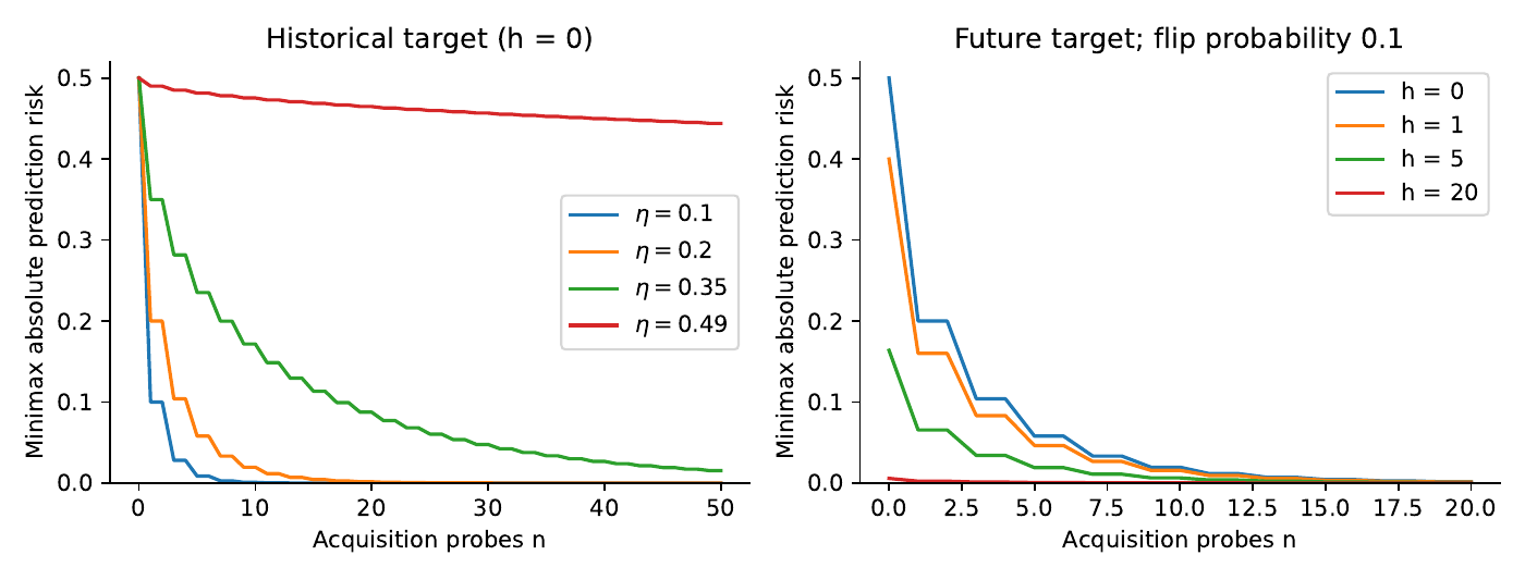
No random seed is needed for these deterministic calculations. The rational dynamic program verifies Bayesian values, and symmetry is what identifies them with minimax values here. That baseline script does not establish minimax equality for asymmetric models; Section 10 supplies a separate asymmetric certification method.
7 Irreversible sensing modes: an adaptive finite-budget frontier
The dominant-channel benchmark removes the reason to adapt. We now resolve one specific instance of the previously proposed mutually exclusive sensing problem. The increment is an explicit finite contract and its exact comparisons; neither adaptive sensing nor belief-state dynamic programming is new.
7.1 Executable protocol and matched comparators
Nature fixes two hidden bits . The mode determines which sensor is useful; the task is to predict , with absolute loss . A controller starts uncommitted with total budget . While uncommitted it may pay one unit for a scout
Alternatively it irrevocably commits to mode . Commitment is a decision with no extra charge. Every remaining unit buys a target reading: BSC of if , or a fresh fair bit if , where . No further scouts or mode changes are allowed. All noises are fresh and independent conditional on and the actions. Exactly paid observations are used. Zero remaining observations permit an arbitrary report. No counterfactual readout from the unchosen mode is exposed.The model label now has four possibilities although the target has two. The good/bad mode is fixed across target readings: marginalizing it produces a mixture of product laws, not an iid BSC with averaged crossover probability. A uniform prior on is used to prove a lower bound; the performance criterion remains the maximum risk over the four fixed parameter values.
We compare: (i) fully adaptive scouting duration and commitment; (ii) a scout count fixed independently of observations, followed by data-dependent commitment and target readings; and (iii) open-loop acquisition actions, including commitment independent of all observations. Terminal prediction may use all acquired data in every class. Private randomization is allowed in every class. These are identical sensor rights and total budgets with different feedback restrictions.
Lemma 7.1 (Risk after commitment). Under the uniform prior, before commitment let . With readings left, the minimum conditional Bayes risk after choosing a mode is An optimizer selects a posterior-most-likely mode and reports the majority of the target readings, randomizing unbiasedly at ties.
Proof. Scouting leaves fair and independent of . For a selected mode with posterior probability of being correct, the target transcript has laws
Their signed difference is , so majority remains Bayes-optimal, including where every report ties. Averaging errors gives , minimized by the largest available . This argument retains the persistent mixture and does not replace it by independent effective noise. ◻Theorem 7.2 (Fixed allocation, adaptive allocation, and minimax). For a fixed integer scout count and , the exact minimax risk is (5) The best open-loop acquisition risk is (6) Define and, for , (7) Zero-probability branches are omitted, avoiding division by zero. The fully adaptive minimax risk is , and Each is symmetric about , concave and piecewise affine. No single posterior threshold structure is asserted.
Proof. For fixed , posterior-MAP estimation of from scouts has error . Conditional on selecting the correct mode the target-majority error is ; conditional on an incorrect choice it is . Lemma 7.1 proves Bayes optimality, yielding (5). These rules have equal risks under all four parameter values, by complementing scout bits and mode labels or complementing target bits and the final report. Uniform-prior Bayes risk is a lower bound on maximum risk, so the equal-risk rule is minimax.
For an open-loop fixed mode and any fixed allocation, under the uniform prior the mode is correct with probability . Scouts can change that posterior probability but cannot change which target-majority decision is optimal: the signed likelihood difference in Lemma 7.1 has the same sign. Averaging therefore gives . Since additional observations cannot worsen optimal Bayes risk, is nonincreasing; hence skipping scouts gives the smallest lower bound. A uniformly randomized mode and majority attain it with equal risks. Open-loop random mixtures of allocations cannot improve an average below its smallest constituent value. This proves (6) for the entire declared class.
Before commitment, the scout posterior , remaining budget , and the known uncommitted permission state are sufficient. Commitment incurs . A scout incurs the second term of (7) by Bayes’ rule and induction. These exhaust the permitted next decisions. Finite horizons and alphabets ensure the minima are attained. Randomization cannot lower a conditional scalar minimum. For each , the expected loss of any fixed finite deterministic policy tree is affine in the initial mode probability ; there are finitely many trees after restricting terminal predictions to endpoint majority rules. Their minimum is piecewise affine and concave. Relabeling the modes proves symmetry.
Finally symmetrize a Bayes-optimal tree over the four transformations generated by mode-complementation and target-bit complementation, with independent uniform private randomness. The protocol and loss are invariant, and this finite group acts transitively on . The transformed rule has the original uniform-prior Bayes risk at each fixed parameter. Thus is attained as maximum risk and equals minimax risk. The inclusions of policy classes give the inequalities. ◻
7.2 A strict gap and a counterexample to cost-unmatched claims
For and , the exact values are
The fixed-allocation risks for are respectively An optimal adaptive rule takes two scouts. If they agree, it commits to their mode and takes three target readings. If they disagree, it takes a third scout, commits to its indicated mode, and takes two target readings. All branches use five paid observations. Under each fixed , its error is (8) The following backward values certify optimality, as distinct from merely constructing an upper bound. Symmetry supplies the omitted complement posteriors; the columns compare immediate commitment with one scout followed by optimal continuation.| Remaining | Mode posterior | Commit | Scout continuation |
|---|---|---|---|
| 1 | |||
| 1 | |||
| 1 | |||
| 2 | |||
| 2 | |||
| 3 | |||
| 3 | |||
| 4 | |||
| 5 |
The additional precision of adaptive scouting is small but strict: its advantage over the best fixed allocation is . Under the uniform prior every scout has zero mutual information about alone, yet scouting can improve subsequent acquisition of . A rule maximizing only immediate information about the target would overlook this instrumental value. This is not a universal failure theorem for information-based design objectives.
Paying for a scout is not always worthwhile. With , and , one scout followed by two target readings has minimax risk , whereas skipping the scout and using three target readings has risk . Holding the number of target readings fixed while adding a free scout would hide this counterexample. At , scouts are wholly uninformative about mode; at , no policy predicts better than .
The stopping in this section concerns the scouting phase; total sample size is fixed. In the terminology of Naghshvar and Javidi [8, Section II-B], this is fixed-size adaptive acquisition, not a variable-total-sample sequential test. The next section treats actual stopping of acquisition.
8 Stopping acquisition when probes have a price
Return to the original binary fixed library of BSCs, now permit a stopping time and charge for each executed probe. The criterion is
The probability target separation remains fixed, independent of stopping and acquisition history. This is an additive cost objective, not a hard expected-budget constraint or a theorem about a moving target. Define for the best channelProposition 8.1 (Standard finite-horizon optimal stopping specialization). Put and again omitting impossible branches. Then the minimax additive objective equals . There is an optimal policy that uses only the strongest channel whenever it continues.
Proof. The stopped-policy simulation uses a fresh strongest-channel observation only when the simulated policy continues, then garbles it as in Lemma 4.1. It reproduces the entire stopped transcript and its stopping-time law under both parameters, including the number of paid probes. Thus weaker channels cannot improve the objective. For the strongest channel, the posterior suffices. Stopping costs and continuing costs the second expression, proving the recursion by backward induction. Reflection and complementing every reading symmetrizes any Bayes-optimal rule to equal total risks under the two parameters. The uniform-prior lower bound is therefore attained as minimax risk. ◻
For , , and , an optimum takes two readings, stops if they agree, and otherwise takes a third. Its error is , its expected sample size under each parameter is , and its objective is . Backward checks are: at and one reading left, stop for ; at and one left, continue for ; at and two left, continue for ; at the initial prior continue for . The best fixed sample count has objective
Randomizing a fixed count independently of observations cannot beat its smallest constituent objective. This exact small example demonstrates a sequentiality gain under a stated price and cap; it does not introduce a new stopping theory.9 Prior art, evidence, and the D04 boundary
The comparison categories and the optimal-stopping machinery have direct antecedents. Naghshvar and Javidi [7, Section 3, Fact 1] give a belief-state stop-or-sense Bellman equation for active hypothesis testing. Naghshvar and Javidi [8, Sections II and IV] distinguish sequentiality from adaptivity and analyze their gains. Li et al. [5, Section III-A, equations (13)–(15)] study finite-horizon stopping and online sensor selection with usage constraints and sampling prices. Our irreversible two-stage permission state and target-only loss differ from their contracts, but a new restricted instance is not a new dynamic-programming principle.
The current search also found the September 2026 revision of Vershinin et al. [15], which addresses unequal and random sensing costs and action cancellation, and Vijayan and Mandal [16], which studies fixed-budget active-testing exponents. These are relevant continuing research lines, not support for a historical-priority claim here. Source editions and inspection depths are recorded in the new source ledger. The search was targeted and is not exhaustive; the precise toy formula’s historical novelty remains unverified.
The original computations were rerun from isolated copies: all 55
transcript checks and nine rational Bayesian-DP checks passed, and both
original data files were byte-identical. The extension script
../code/verify_extensions.py independently optimizes a full
posterior on all four
states, without invoking Lemma 7.1 inside that
oracle, and agrees exactly with the scalar recurrence on 200
parameter/horizon combinations. It independently checks the
fixed-allocation formula against a constrained full-state oracle in 900
cases. It also directly enumerates paths of the displayed five-probe
policy under every parameter, verifies all fixed allocations, the budget
counterexample, and the total-stopping example. A separate specialist
wrote a second exact rational recursion and statewise policy
calculation. These are bounded computational checks, not formal proof
verification. The printed arguments establish the model-level results;
no empirical sensor data were used.
D04’s finite-library theorem assumes paid common validation episodes that can acquire the union of candidate tests. The mutually exclusive sensors here violate that assumption; observing a scout and one selected sensor does not produce the counterfactual outputs of all modes. This gives D04 an executable boundary example, not a coupled representation-selection theorem. The bits, candidate modes and noise laws are supplied and fixed here. Nothing learns a new representation language, estimates the channel laws from paid labels, prices its code, or optimizes representation-revision costs. The useful handoff is to retain D02’s acquisition/permission state and D04’s validation/revision charges in a future joint model. Merely renaming a mode a concept does not prove that joint result.
10 Beyond symmetry: executable minimax certificates
The preceding exact frontiers exploit symmetric channels and equalizer policies. An asymmetric nuisance parameter removes that shortcut. This section supplies a general finite certification contract and a larger asymmetric benchmark. The underlying methods are finite zero-sum game duality and belief-state control, not new minimax principles. Their purpose is to make the computational claim checkable without assuming a uniform prior is least favorable.
10.2 An asymmetric example with a complete small certificate
Use the two-mode irreversible protocol with , but let
and give the correct sensors crossover probabilities in mode zero and in mode one. A wrong-mode sensor remains fair. A scout followed by a target reading, with and , has bit-symmetric mode risks Choosing , makes both risks . Execute this by mixing “choose mode ” with weight and “always choose mode one” with weight , after the scout. This is a feasible upper certificate.For the lower certificate use prior on . If the first action commits to a target sensor, the second must use that sensor. The two-read mixture retains the majority sign and , so prior risks for fixed modes zero and one are and . If the first action scouts, the posterior mode-zero mass after is , making the two modes tied at target risk ; after it is , favoring mode one. Averaging yields . A second scout without any target reading leaves error . These exhaust the legal first-step choices and their optimal continuations, proving the lower bound and hence the exact minimax value .
By contrast, the uniform-prior Bayes policy selects mode and has average error , but worst error . The best open-loop policy has minimax risk . The latter follows by mixing fixed modes zero and one to equalize and at ; independently sampled scouts do not improve the optimal majority decision for a fixed mode. The independently written specialist script also exhaustively enumerates all 176 deterministic legal two-step trees, including every terminal decoder, and verifies both lower certificates. This small result is a regression test for the general method, not a priority claim.
11 An asymmetric six-candidate reproducible study
To avoid simply increasing the size of the symmetric example, let , , with six fixed candidates and target . Scout has three outputs, with rows indexed by :
The three binary target sensors have probabilities of output one as follows. Every printed decimal is an exact rational hundredth or tenth.| Sensor | ||||||
|---|---|---|---|---|---|---|
| .08 | .88 | .30 | .55 | .42 | .60 | |
| .25 | .60 | .18 | .82 | .35 | .52 | |
| .33 | .65 | .40 | .58 | .12 | .75 |
All outcomes are fresh conditional on and actions. Cross-mode sensors are informative, no bit-reflection symmetry is assumed, and the channels cannot be replaced by the good/fair mixture formula. Before commitment the learner may scout or take a target reading. Taking the first target reading commits to its sensor, after which only that sensor remains available. Every observation costs one and total count is fixed at ; commitment has no separate free observation. The tables are invented synthetic laws, not empirical sensor calibration, biomedical validation, or evidence of practical savings.
The open-loop comparator randomizes over legal schedules independently of outcomes and may decode using the full observed transcript. Legal schedules are , including all scouts. The reversible comparator may use any sensor or scout at any step and has explicitly greater action rights; it isolates the value of relaxing irreversibility, not an architecture advantage. All classes use the same terminal target, sample count, known laws and private randomization.
11.1 Certificates, executable policies, and negative controls
The solver repeatedly asks a Bayesian dynamic program for a best-response tree to a candidate prior and adds its candidatewise risk vector to a finite-game LP. Floating-point LPs propose priors and mixtures; their active systems are reconstructed over the rationals. An exact Bayes recursion then computes the lower bound and an executable mixture’s risk gives the upper bound. If reconstruction fails, rationalized feasible candidates still give an enclosure; equality is never inferred from solver tolerance. The saved policy is a directed acyclic graph of actions, observation branches and terminal reports. It receives observations and its own random mixture choice, never a hidden state label.
All 17 reported cases have exactly zero rational certificate gap. The independent verifier reads only the saved model/policy/certificate, checks legal action sequences and horizon, evaluates candidatewise policy risks, and independently recomputes the Bayes lower bound without the optimizer or its oracle. The small asymmetric example supplies a separately enumerated control. The certificate checks are algorithmic verification under supplied kernels, not formal proof-assistant verification.
| Irreversible adaptive | Open-loop | Reversible adaptive | |
|---|---|---|---|
| 0 | .500000000 | .500000000 | .500000000 |
| 1 | .330151462 | .330151462 | .330151462 |
| 2 | .268760234 | .306356429 | .268619242 |
| 3 | .231259259 | .257860485 | .224222209 |
| 4 | .176811713 | .235287802 | .176125933 |
| 5 | .157907608 | .213936487 | not computed |
These are rounded exact minimax values for the declared finite instances. At the irreversible value is
Its stored optimal mixture has six trees, with a combined 34-node graph including the separate uniform-prior baseline. All six candidatewise risks equal this fraction. The selected deterministic uniform-prior Bayes rule has worst risk . This reports that specific tie-broken rule, not a claim that every possible uniform-Bayes tie resolution has that worst risk. The exact primal/dual certificate is the reason to call the returned mixture minimax.The adaptive advantage over open-loop at is about ; the extra advantage of reversible rights is only . The latter small positive gap should not be advertised as a robust practical effect. A gap’s magnitude, not only its sign, matters when the model is approximate.
12 Model mismatch and the limits of the numerical advantage
Proposition 12.1 (Common-contract finite-horizon coupling bound). Let and have the same candidates, initial laws, finite alphabets, initial permission, legality map, horizon and terminal loss in . Suppose for every candidate and legal , where the compared outcome includes . Put . Every fixed policy’s candidatewise risks change by at most , and A policy certified on by bounds has worst risk at most on and regret at most . The true minimax value lies in , clipped to .
Proof. Couple equal initial latent states and the same private policy randomness. While latent states and complete observed histories agree, the selected actions agree and are legal. Maximal coupling of the next joint outcome preserves equality with probability at least . Induction gives probability at least of agreement through the horizon. On that event the report and loss agree; elsewhere their difference is at most one. This proves the policywise risk bound. Maximum and infimum preserve uniform bounds, proving value sensitivity. For the transferred policy, its risk is at most , while the true optimum is at least ; subtract. The bounds concern a fixed perturbed candidate family, not a reselected hidden parameter at every history. ◻
This is a standard finite coupling/simulation bound. Explicit POMDP model and transferred-policy sensitivity have substantial primary antecedents [2]; recent policy-observation robustness work explicitly separates fixed from history-dependent model deviations [4]. Costed switching [14] and usage-constrained sensing [5] also predate this note. Our result does not replace their richer models or establish a new general robustness theory.
The common-contract condition is necessary. If a first action has identical readout under two systems but irreversibly disables a later informative sensor in only one, readout-only total variation at that step is zero while the future executable policy sets differ. Comparing the joint permission successor exposes that difference; silently changing legality makes policy transfer undefined. Changes in target loss need a separate discrepancy term. The terminal-loss theorem does not retain its constant for unbounded cumulative costs.
For the six-candidate study, suppose externally justified common-contract kernel error is at most . At , . Applying the theorem separately to the two policy classes preserves an adaptive-over-open-loop value gap of at least . By contrast, even gives , larger than the reversible-rights gap; this certificate is inconclusive about its persistence. This does not prove that the small gap reverses. At , the bound also becomes inconclusive for the larger adaptivity gap.
We additionally perturb all binary target probabilities by , toward or away from ambiguous target responses, and evaluate the frozen nominal policy exactly; the scout kernel is unchanged. These are eight structured perturbations per certificate, not optimization over every allowed perturbed family. For irreversible , moving probabilities toward ambiguity raises worst risk from to at , at , and at . All 136 saved stress checks obey the coupling bound. No observed data establish that any real sensor satisfies these error radii. Obtaining such a bound requires a separately specified calibration experiment and its costs; a deployment learner cannot inspect for free.
13 What improved, and what still needs human judgment
The larger contribution is not the mere use of more states. The revision removes the symmetry-based identification of Bayes with minimax, supplies executable policy/lower-bound certificates, proves the required common-interface transfer bound, and records when the apparent advantage is too small for that bound to protect. It retains the simpler exact examples as transparent controls. The prior-art audit strengthens attribution and may reinforce, rather than improve, the weak evidence for historical novelty.
For human feedback, the useful questions are specific: does the irreversible-permission certificate/benchmark illuminate an existing sequential-design problem; which historical experiment-selection or nuisance-testing literature subsumes the construction; and what physically measured irreversible interface would justify an empirical study? The next mathematical work should treat learned channel laws or a coupled paid-validation contract, with confidence sets and a fixed versus adaptive uncertainty convention stated explicitly. The present methods note supplies neither a scalable general algorithm nor empirical validation, and no theorem about D04’s endogenous representation learning follows.
14 Unresolved investigation and portfolio relation
Precisely unresolved problem.
The new scout-and-commit family resolves one specific fixed-mode, fresh-noise case, not general constrained stochastic acquisition. The finite permission-state certificate now covers supplied finite hidden controlled models, without providing a closed frontier or scalable algorithm. Unknown channel reliability, statistically learned uncertainty sets, arbitrary unbounded histories, and coupled paid-validation/representation revision remain unresolved. Any state reduction or approximation still requires a certificate.
D02 versus D04.
This note holds the evaluation target fixed and asks what an interface can acquire. D04 chooses among representations using task performance and paid distinctions. Its selection theorem is not the same theorem as the channel frontier, although a representation-selection experiment can use this frontier as a lower-bound subproblem. If a future D04 manuscript merely selects among these three channels, it should be merged into this note. The present drafts retain distinct decision variables.
Being, Becoming, and The MIND.
The operational content of Being is the predictive capability available under a present experiment budget. Becoming is an alteration of that capability through observations or changes to the interface. A model-based agent can also recognize a task-relevant ambiguity and refrain from claiming identification. These are useful functional targets. They do not establish phenomenal consciousness or a discovered self/world boundary.
Publication assessment.
The solved benchmark, explicit timing, and failure cases suit a methods appendix to the acquisition/diagnosis line. The new exact examples strengthen the methods material but do not verify standalone novelty. A separate submission would need a broader priority audit and assessment of whether the restricted family adds a substantive result beyond established controlled sensing. The existing acquisition and diagnosis notes remain the closest internal antecedents.
References
- Henrique de Oliveira. Blackwell’s informativeness theorem using diagrams. Games and Economic Behavior, 109:126–131, 2018. doi: 10.1016/j.geb.2017.12.008. URL https://henriquedeoliveira.com/wp-content/uploads/2020/12/blackwells-informativeness-theorem-using-diagrams.pdf. Author preprint dated 30 November 2017; relevant Theorem 1 and Section 4 read. Journal metadata verified against publisher and institutional record. Accessed 13 November 2026.
- Yunus Emre Demirci, Ali Devran Kara, and Serdar Yüksel. Sensitivity of filter kernels and robustness bounds to transition and measurement kernel perturbations in partially observable stochastic control, 2025. URL https://arxiv.org/abs/2508.10658v3. v3, 12 September 2025. Latest abstract and selected passages inspected. Earlier v1 Section 6.2 was read separately under its earlier title; no full-proof audit.
- Wassily Hoeffding. Probability inequalities for sums of bounded random variables. Journal of the American Statistical Association, 58(301):13–30, 1963. doi: 10.1080/01621459.1963.10500830. URL https://www.cs.rpi.edu/academics/courses/spring06/random/hoefding.pdf.
- Benjamin Kraske, Qi Heng Ho, Federico Rossi, Morteza Lahijanian, and Zachary Sunberg. Robustness analysis of POMDP policies to observation perturbations, 2026. URL https://arxiv.org/abs/2604.21256v1. v1, 23 April 2026. Abstract and Sections 2.3 and 3 inspected; fixed/history-dependent uncertainty distinction.
- Shang Li, Xiaoou Li, Xiaodong Wang, and Jingchen Liu. Sequential hypothesis test with online usage-constrained sensor selection. IEEE Transactions on Information Theory, 65(7):4392–4410, 2019. doi: 10.1109/TIT.2019.2910730. URL https://arxiv.org/abs/1601.06447v1. Read 2016 primary preprint Sections I–III-A, especially equations (13)–(15).
- Michael L. Littman, Richard S. Sutton, and Satinder Singh. Predictive representations of state. In Advances in Neural Information Processing Systems, volume 14, pages 1555–1561, 2001. URL https://papers.neurips.cc/paper_files/paper/2001/file/1e4d36177d71bbb3558e43af9577d70e-Paper.pdf.
- Mohammad Naghshvar and Tara Javidi. Active sequential hypothesis testing. The Annals of Statistics, 41(6):2703–2738, 2013. doi: 10.1214/13-AOS1144. URL https://arxiv.org/abs/1203.4626v4. Section 3, Fact 1 read in the primary arXiv reprint; not a full proof audit.
- Mohammad Naghshvar and Tara Javidi. Sequentiality and adaptivity gains in active hypothesis testing. IEEE Journal of Selected Topics in Signal Processing, 7(5):768–782, 2013. URL https://arxiv.org/abs/1211.2291v1. Read primary 10 November 2012 preprint, especially policy categories in Section II-B.
- Sirin Nitinawarat, George K. Atia, and Venugopal V. Veeravalli. Controlled sensing for multihypothesis testing. IEEE Transactions on Automatic Control, 58(10):2451–2464, 2013. doi: 10.1109/TAC.2013.2261188. URL https://vvv.ece.illinois.edu/papers/journal/niti-atia-veer-tac-2013.pdf.
- Research development draft prepared for Brian Theory. Causal self-diagnosis with noisy tests: Observation laws, irreversible access, and task recovery, 2026. URL https://www.b-theory.com/manuscripts/causal-self-diagnosis-r1-v0.3-2026-11-05.pdf. Version 0.3, 5 November 2026. Original submission authorship unresolved; fixed 38-page reading copy. Accessed 13 November 2026.
- Cosma Rohilla Shalizi and James P. Crutchfield. Computational mechanics: Pattern and prediction, structure and simplicity. Journal of Statistical Physics, 104:817–879, 2001. doi: 10.1023/A:1010388907793. URL https://arxiv.org/abs/cond-mat/9907176. Read in arXiv:cond-mat/9907176v2; relevant source locators are Definition 5 and Section V.
- Richard D. Smallwood and Edward J. Sondik. The optimal control of partially observable markov processes over a finite horizon. Operations Research, 21(5):1071–1088, 1973. doi: 10.1287/opre.21.5.1071. Publisher metadata and abstract checked; full original proof not re-audited.
- Brian Theory. From observable states to acquirable predictive models, 2026. URL https://www.b-theory.com/manuscripts-html/acquirable-predictive-models/. Revised technical report, 7 October 2026; site reading copy 1. Accessed 13 November 2026.
- Nidhin Koshy Vaidhiyan and Rajesh Sundaresan. Active search with a cost for switching actions, 2015. URL https://arxiv.org/abs/1505.02358v1. Read primary v1, 10 May 2015; abstract, introduction and model context. Asymptotic proofs not audited.
- George Vershinin, Asaf Cohen, and Omer Gurewitz. On cost-aware designs for sequential hypothesis testing, 2026. URL https://arxiv.org/abs/2512.19067v3. arXiv:2512.19067v3, 24 September 2026. Abstract, introduction and model scope inspected; proofs not audited.
- Sushant Vijayan and Himadri Mandal. PDE-based bounds on optimal exponents in active simple hypothesis testing, 2026. URL https://arxiv.org/abs/2610.36657v1. arXiv:2610.36657v1, 27 October 2026. Abstract and Sections I–II inspected by the independent reviewer; proof audit not claimed.