When to Split and When to Merge
Task-driven observation concepts with paid audits and repeated
revision
AI-assisted research draft
13 November 2026
D04 — Revised technical methods note, version 2. Finite-class and anytime guarantees use standard tools. Exact Bayesian models price validation, deployment and revision separately. A hidden-regime extension permits repeated revision while tasks continue. Open-ended concept development remains unresolved; no general novelty claim is made.
Abstract
A representation should retain distinctions that improve a declared task enough to justify their acquisition, memory, and revision costs. We study a finite library of representations computed from observable histories, with supervised feedback obtained through a paid validation protocol. For all compatible finite decision tables, we derive a simultaneous risk certificate, a penalized selection bound, and conservative split/merge rules. An elementary total-variation bound quantifies the task loss caused by merging prediction classes. A two-regime binary example has an exact threshold for keeping a noisy feature, and revision costs create a transparent hysteresis interval. A transfer guarantee requires an explicit bound on the change of the observable task distribution; usefulness on one task alone is insufficient. Reproducible experiments show both the benefit and delay of confidence-gated revision relative to ordinary penalized empirical-risk selection. These results implement a modest operational sense of changing concepts, while the central mathematics remains finite-class learning and decision theory. We extend validation to predictably allocated partial-coverage streams with an anytime certificate, then solve an exact two-query Bayesian stopping example in which nonmyopic acquisition is worthwhile although one-step information value is zero. The installed representation changes the acquisition price threshold. A recurring-task extension permits repeated revisions under hidden regime changes, gives hysteresis and perturbation bounds, and is solved by exact rational policy envelopes. Full sensitivity and frozen-policy tests retain zero-benefit and harmful cases. These are standard-method specializations, not a general concept-development theorem.
1 The question and the current B-Theory baseline
A supplied refinement tells an observer which distinctions a representation contains. It does not specify how a learner discovers that a distinction is useful, when the available evidence warrants introducing it, or when to remove it. Those decisions require a task, an observable experiment, and a cost model.
The current Successive Concept Differentiation as Observation Refinement, referee-repair v0.5 dated 29 September 2026, distinguishes signature refinement, carrier splitting, and order thinning. Its Section 6 defines refinement of observation maps; Sections 7–9 study a supplied Boolean observation’s structural effect [14]. This note instead chooses a representation from data. It does not replace the structural theorems or prove that a homology change improves a task. The site’s separate General Observation Refinement material is explicitly unfinished and retracts a former observation-dimension equality; no result here depends on that equality.
External precedents and novelty boundary.
State abstraction has a long history in control and learning. Li et al. [7, Section 3] distinguish several preservation objectives for finite MDP abstractions; their abstraction definitions concern ground-state models. Their Section 2 and Table 1 also describe statistical online aggregation and disaggregation, including methods that do not require a supplied MDP model. Thus data-driven splitting and merging itself is an established idea. Approximate MDP metrics can link changes in dynamics and rewards to value differences [3, Sections 4–5]. Our observable one-step supervised contract is more limited: the learner is never permitted to inspect the latent regime, and we prove no MDP value guarantee. Oudeyer et al. [9, Section III] distinguish error seeking from learning progress and discuss the trap of unpredictable noise. Choosing a paid feature by finite-class validation is not a new theory of intrinsic motivation. The value is an inspectable contract combining acquisition, split/merge decisions, and revision costs; this combination is not asserted historically novel. Sections 9–10 add sequential validation and directly compare costly active model selection and feature-acquisition precedents.
2 What the learner can actually observe
2.1 A finite language and a paid validation channel
Let be a finite space of observable histories and a finite feedback alphabet. A validation episode first produces a history , then returns a task label according to an unknown law on . The label is supervised feedback available to the learner, not the hidden regime used to generate an illustration. It does not depend on the learner’s prediction in this model. Thus a complete labeled episode can evaluate several candidate predictions on the same example.
Before seeing validation data, specify a finite library of maps . Each map must be implementable from declared sensor tests. The validation protocol is permitted to acquire the union of these tests; it pays the resulting observation cost. During deployment, the selected representation obtains only the tests it requires. This complete-information validation assumption is strong. If two tests are mutually exclusive, destructive, or available only after different state-changing actions, the present common validation sample is not automatically executable. A bandit or controlled experiment model is then required.
For finite actions , a candidate is a pair with . Its prediction is . Let be the specified finite set of candidates and . One may include every compatible action table, giving
This count concerns code alternatives as well as partitions. Selecting a partition and then fitting its actions on the same data is covered only if all the resulting tables are included in the uniform class, or if fitting and validation use independent samples.2.2 Risk, resources, and a fixed evaluation block
Loss satisfies . For a candidate define
Here is the currently installed candidate, is its known recurring cost per deployed decision, is the known one-time revision cost with , and is the common evaluation block length. Costs are already converted to the same units as loss using explicit designer weights. They may include sensor acquisition, retained bits, computation, and a readout table. A count of representational states is not automatically the number of physical memory bits; if fixed-length storage is used, at least state bits are required, with code and precision counted separately.All candidates receive the same information about costs, task, library, and labeled validation episodes. The common training cost is paid by every data-driven comparator and should be added as to a full lifecycle objective. It cancels from selection within a fixed validation batch, but it does not disappear when comparing different sample sizes or comparing validation with immediate deployment. The theorems below optimize selection conditional on the declared batch; they do not establish that the batch itself was worth buying.
Within a validation/deployment block, is stationary and validation pairs are independent and identically distributed. No hidden state is supplied to a candidate. The finite language is fixed before validation. Choosing a feature from this library is not inventing a new sensor or extending the language.
3 A useful distinction is task dependent
Definition 3.1. A representation refines if for a map . Let be the smallest risk among all action maps on .
Proposition 3.2 (Unpriced refinement). If refines and every coarse action table may be lifted to the fine representation, then .
Proof. For each coarse table , the fine table makes exactly the same decision at every history. The fine policy class therefore contains a copy of the coarse class; minimizing over it cannot increase risk. ◻
The proposition concerns optimal task risk with free observations and free tables. It does not imply that improves, that a finite learner will find the improved table, or that more distinctions are developmental progress. The entire gain can be zero.
Proposition 3.3 (Task loss caused by merging). Suppose . For a fine class of positive probability let be the conditional law of given , and let be the conditional law in its coarse class. Then Zero-probability classes contribute zero and require no conditional law. In particular, if every displayed distance is at most , a recurring saving exceeding plus amortized revision cost suffices to justify the merge when both candidates use their Bayes-optimal action tables. The bound alone does not certify an arbitrary fitted coarse table.
Proof. For a distribution on labels, write . Since losses lie in , for every action . Evaluate each minimum using an optimizer of the other to obtain . The coarse conditional law is the mixture of its fine laws. Therefore
is bounded above by the stated sum. Nonnegativity follows from Proposition 3.2. Subtract the recurring saving and add the one-time cost divided by to compare objectives. ◻This is an elementary decision-risk bound, not a new abstraction theorem. It preserves the specified label-prediction task. It does not promise preservation of causal interventions, historical facts, or an unrelated future task. D06 addresses those stronger preservation contracts.
4 Evidence sufficient to authorize a revision
Given validation examples, set
Replace by in to obtain . All logarithms in this section are natural.Lemma 4.1 (Bounded empirical means). For independent variables with a common mean, the probability that their average differs from its expectation by more than is at most .
Proof. This is the specialization of Hoeffding’s inequality [4, Theorem 2, equation (2.6)]. A short reconstruction is useful. Let for one bounded variable. Under exponential tilting, is a variance and is at most : . Since and , twice integrating gives . Independence multiplies moment-generating functions. Exponential Markov inequality bounds the upper tail by , minimized at . Apply the same argument to and sum the two tails. ◻
Theorem 4.2 (Finite-library selection and a revision certificate). With probability at least , simultaneously for every , On that event:
A minimizer of satisfies .
If , replacing by strictly improves the true block objective.
A switch from to is certified whenever .
Proof. Apply Lemma 4.1 to each fixed candidate and take a union bound over . Known costs add no estimation error. For the first claim, if minimizes , then
For the second, . For the third, the empirical difference is at least the true difference minus , and hence exceeds the switching threshold. ◻A confidence-gated rule computes the empirical minimizer but retains unless the second inequality holds. It has a useful no-harm certificate on the confidence event, but it does not inherit the first claim’s oracle bound unchanged. If the gate does not switch, comparison with gives the looser bound . The delay in acting on a small real gain is a genuine cost, illustrated below.
Splits and merges use the same certificate.
For a proposed split, the empirical task improvement must exceed the extra recurring cost, the amortized revision cost, and . For a proposed merge, the recurring saving must exceed the estimated task deterioration, revision cost, and . A high-entropy feature, an unexpected observation, or a visible topological change is not itself evidence satisfying either test.
Repeated decisions.
At decision block , permit the candidate class to depend on past data, but require it to be fixed before a fresh conditionally iid validation batch. Use failure allowances with . Conditional application of the theorem and a union bound give simultaneous valid certificates for those blocks. This construction does not detect a change within a block. Reusing one holdout indefinitely while adaptively inventing candidates violates the conditional-fixed-class premise.
5 A lower bound on detecting a useful split
The ability to list a feature does not make its task value immediately knowable. Consider a fair observable bit and a label . Under , is an independent fair bit. Under , , with . In both models and are marginally fair. A coarse constant predictor has risk . The predictor has risk under and under . Give the feature a recurring cost and no revision cost. Coarse is better in the first model and fine is better in the second.
Proposition 5.1 (Necessary evidence scale; elementary two-point bound). Any procedure selecting the better representation with error at most under both models from iid labeled pairs must satisfy
Proof. Selecting fine versus coarse defines a binary test. The sum of its two error probabilities is at least : for its acceptance event , the sum is . Moreover,
using and the four joint atom probabilities. Additivity of KL over independent samples and the finite Pinsker inequality give . Hence and rearrangement proves the bound. Pinsker itself follows by grouping the positive likelihood-difference event and using the binary KL second derivative . ◻This only establishes a necessary inverse-square scale; it is not a sharp sample-complexity theorem. Its testing argument also occurs in D02, which should be cited as a shared method in a combined presentation rather than counted as a separate research contribution.
6 A solved split/merge example
Let an unobserved regime be a fair bit. A paid test returns with , and supervisory feedback is with . The noises and are independent; . The learner sees only in validation. The latent is used by the analyst to define the data-generating model, never by the learner’s rule.
The coarse representation is constant and the fine representation retains . Under zero-one loss,
To verify the fine risk, note that exactly when one of the two noise bits flips. Symmetry makes the optimal prediction when . If fine has extra recurring cost and a coarse-to-fine revision costs , splitting for a block of length is favorable precisely when The inequality is strict because a tie provides no strict advantage. Choosing either candidate at a tie gives the same objective.Now let be the net recurring advantage of fine, and assume a symmetric switching cost between the two installed models. A controller committing for one common -decision block switches coarse to fine iff , and switches fine to coarse iff . The interval is a hysteresis region in which keeping the current representation is optimal for this block. This is an exact two-choice calculation, not a globally optimal policy for an unknown changing future.
In a later task, make independent of . Both representations have best task risk , so positive recurring feature cost favors a merge once its saving exceeds revision cost. A permanently growing representation is then suboptimal. An unrelated independent noise bit has the same one-bit entropy as but supplies no prediction benefit at any cost; representation variability is therefore not the objective.
7 Transfer requires a quantitative relationship
Proposition 7.1 (Distributional transfer certificate). Let and be laws on the same observable-history and label space with , the same loss function and costs. Then for every fixed candidate. If , the replacement still improves the objective under . Combined with the validation event, the sufficient empirical threshold is .
Proof. A fixed candidate’s loss is a -valued function of , so its expectation changes by at most total variation. Costs are unchanged. Apply this bound to both candidates and use Theorem 4.2 for the empirical version. ◻
This guarantee is useful only if is justified independently or estimated under a further valid experiment. It cannot be inferred just because two tasks share vocabulary. If the label map or loss changes, that change must be encoded in a shared augmented task variable or bounded separately. A feature that perfectly predicts the first label may be independent of the second. No universal transfer claim follows from refinement alone.
8 Reproducible study: certificates can be expensive
The script code/reproduce.py implements the four
observable prediction tables
.
Training data consist only of counts of the four
pairs. All policies have the same labeled data, and recurring costs are
.
We compare ordinary penalized empirical risk minimization with the
confidence gate at
,
using 20,000 independent training batches for each sample size and
regime, seed 20261113. The two fixed baselines are coarse risk
and fine objective
;
a known-distribution oracle chooses their minimum. Test risk after a
selection is evaluated analytically from the generating law, so
simulation variability is solely over training samples.
In the useful regime , so and the optimal objective is . At , the gate retains the feature in of batches and has mean objective , whereas penalized empirical risk selects the feature in all 20,000 sampled batches. In the irrelevant regime , starting from fine, the gate still retains a feature in of batches at , although the oracle merges. At that fraction is . These are observed finite simulation proportions, not exact probabilities or failure-rate bounds. The conservative certificate trades responsiveness for a stated high-probability improvement guarantee.
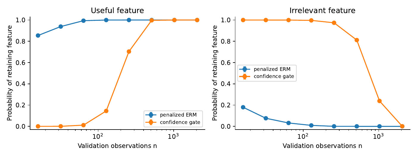
The code also checks the merge inequality for 4,851 two-component Bernoulli mixtures on a finite grid. It records all parameters, selection counts, standard errors, data, and figure sources. The grid corroborates the implementation, while Proposition 3.3 supplies the general proof. The study is not a benchmark against modern representation learning on real data; its role is to expose the consequence of the certificate under the minimal model.
9 Sequential paid validation with partial coverage
The preceding fixed-batch theorem does not justify monitoring its interval until a favorable result appears. We now allow adaptive allocation and stopping under an explicit, narrower-than-general-active-learning interface. The following construction is elementary error spending; sharper confidence sequences are available [5, Section 1 and equation (1)].
Fix a finite experiment set . Experiment costs and reveals losses only for a fixed nonempty subset . Its th invocation exposes the next entry of an iid vector stream with for each . Independent streams are a sufficient implementation; dependence among candidates in one vector is allowed. The controller chooses using previously exposed data, before seeing the fresh episode. No hidden regime, unqueried feature or label is supplied. Every query is charged once even if it evaluates several candidates. Costs of mutually incompatible tests are never replaced by free joint observation. The class and all coverage sets are fixed in advance, and the target distribution remains stationary. Different experiments estimating a candidate must estimate the same deployment risk, not selected subpopulation risks.
Write and let be a stream-prefix average. For and , set
At any global time, intersect with all available intervals for that candidate, obtaining . Unsampled candidates receive . An empty intersection is a diagnostic failure; the specified certificate rule returns and abstains from a certificate based on that inconsistency.Theorem 9.1 (Anytime partial-coverage revision certificate). With probability at least , every interval at every time contains its candidate’s risk, under every predictable adaptive experiment-allocation rule and every stopping rule. On this event the data-dependent switch strictly improves its common -decision block objective whenever For a sequence of such certified switches in the same stationary model and at the same , put . No candidate is revisited, so at most switches occur. For every nonempty finite prefix ,
Proof. For each fixed Hoeffding gives failure probability at most . Summing over the covered pairs and using proves a single event containing every stream prefix. Adaptive allocation exposes prefixes of these same streams; it does not change that event. Intersections contain the true risk on the event, including at random times. The switch inequality implies . Strict descent of the fixed function excludes repetitions in the finite class. Summing the strict inequalities proves the cost statement. ◻
This is a safety certificate for the deployed block comparison, not a bound on the complete acquisition bill . It neither chooses an efficient experiment allocation nor establishes that querying was worth its cost. The telescoping statement is a potential bound, not accumulated deployment regret. Stationary fixed is essential: task changes can legitimately cause returns to a previously used representation. These frequentist guarantees also remain separate from the Bayesian optimization below.
A concrete selection-bias counterexample.
Let be fair, , and . Its target risk is . If a controller sees the current for free and purchases a label only when , every recorded loss is zero. Stream averaging estimates zero rather than , regardless of sample size. Our theorem therefore excludes outcome-dependent filtering and general context-dependent query selection without an appropriate sampling correction. Merely having a large sample or an anytime radius does not repair this mismatch.
10 When is another paid query worth buying?
10.1 Finite prior, fixed deployment block, optional stopping
Let belong to a finite set with known prior . Conditional on , a fresh query of experiment has known finite outcome law ; conditional on and the previously exposed history, the next outcome after selecting has law . The learner observes only the purchased outcomes and updates its posterior. Known candidate risks are functions , with fixed deployment and revision charges. The unknown itself is never revealed.
At most queries may be purchased before committing to a representation for the same subsequent deployment tasks. Queries do not consume those tasks, change , or change their distribution. Their price includes acquisition and feedback. No deployment labels or realized losses feed back into learning, and unlabelled observations in the example below are ancillary. There is one terminal installation decision. This is adaptive validation followed by revision, not a solution to interleaved online revision, drift, or language expansion. Posterior computation, code storage and planning are not optimized; all policies receive the same model information and interface.
For currently installed , define
With predictive outcome law and Bayes update (zero-probability outcomes omitted), the total lifecycle value is (1)Proposition 10.1 (Declared finite-model optimum). Equation (1) minimizes the expected sum of all query charges, terminal revision cost and deployment losses and recurring charges over every admissible adaptive randomized policy.
Proof. With no queries left, conditional expectation gives . At positive depth the first action either commits, or purchases one experiment, incurs its charge and observes its outcome. The posterior is sufficient for the remaining conditional law by the model assumptions. Induction gives the optimal continuation at each outcome. A randomized first action averages these costs and cannot beat their minimum. The finite action and outcome sets attain every minimum. ◻
This is standard finite-horizon Bayesian decision theory, not a new Bellman principle. Costly model probes, posterior policies and budget-sensitive strategies already occur in active model selection [8, Sections 2–3]. Active sensing already optimizes error, delay and repositioning costs [1]; joint feature acquisition and classification is established [12]. Recent incomplete-training-data work explicitly uses truncated acquisition Bellman recursions [11, Section 3.2, equation (4)]. The purpose here is to expose the installed-representation charge and distinguish query cost from recurring deployment cost in an exactly auditable example.
10.2 An exact two-query frontier, including the installed state
Let be static with prior . Each validation episode returns a fair feature and label , where the mismatch probabilities are and . Within an episode and are independent conditional on ; fresh pairs are also independent across episodes conditional on . Coarse predicts zero with risk ; fine predicts its paid feature with risk and recurring cost . Coarse cost is zero. The fixed library contains these two candidates; no additional fitted tables are introduced. Set , symmetric nonzero revision cost , and at most two validation episodes at price apiece. Each deployed fine prediction buys a fresh feature; that expense is already in . There is no free supervised deployment feedback.
With posterior , the two stopping envelopes are
Thus coarse splits at and fine merges at ; ties allow either action. The intervening interval is the one-block installed-state hysteresis region, not an infinite-horizon switching theorem. Write for , a directly observable validation event. The predictive probabilities and posteriors are After or the posterior is , and after it is .Theorem 10.2 (Two-query price frontier). For either incumbent one query has zero expected reduction in the optimal stopping cost before charging its price. With up to two queries, the exact values at prior are Consequently, buying evidence strictly improves the Bayes lifecycle objective iff from coarse, or from fine. Below the relevant threshold an optimal policy queries once, stops at the first mismatch, and queries again after a first match. It deploys fine only after two matches and deploys coarse otherwise. At a threshold, immediate stopping and that query policy tie.
Proof. Both one-query posteriors are below and , so coarse is the stopping choice after either outcome for both incumbents; its cost is constant. This proves zero one-step information value. With two queries, the only leaf where fine is chosen is . After an initial mismatch even a subsequent match cannot change the stopping choice, so a second query there has zero value and can be omitted. Conditional on a first match, the prospective terminal savings times its probability at the root are
The query policy uses episodes in expectation. Its terminal cost is the immediate stopping cost minus the displayed saving, giving the two affine expressions. It beats stopping exactly at the stated prices. At any such price, the second query after a match is also beneficial: its conditional saving is the displayed root saving divided by , which exceeds the root break-even price (the same saving divided by ). If that second query is not beneficial, buying only the first cannot help; if it is beneficial but the whole policy is not, stopping is optimal. These exhaust the Bellman alternatives. At , additional useless queries are harmless ties. ◻| Incumbent | Immediate stop | Mandatory two, | Adaptive, |
|---|---|---|---|
| Coarse | 5 | 4.9945 | 4.991 |
| Fine | 5.1 | 5.0055 | 5.002 |
For coarse at , adaptive acquisition costs , whereas a mandatory two-query policy costs and immediate stopping costs . Thus an entire price interval makes adaptive validation worthwhile when committing to two queries is not. This is a small declared-model example of nonmyopic option value; nonmyopic acquisition and failures of one-step lookahead are established phenomena, not discoveries claimed here.
Bayes benefit does not mean pointwise safety.
At and coarse incumbent, the optimal query policy costs under and under , averaging . It harms the bad environment relative to the no-query cost . A posterior-optimal revision therefore does not inherit Theorem 9.1’s high-probability true-risk certificate. Misspecified priors or likelihoods can invalidate the Bayesian comparison. This explicit counterexample prevents conflating expected value of learning with distribution-free no-harm.
Reproducibility and scope.
The script code/sequential.py uses exact rational
arithmetic for the Bellman recursion and independently enumerates all
deterministic trees of depth at most two, with query or terminal
deployment actions. It checks both incumbents over a price grid
including both exact thresholds and exports exact fractions, expected
costs and policy decisions. Enumeration tests this finite example, while
the displayed proof establishes the price formulas. No simulation,
asymptotic claim, real-world performance result, or sensor invention is
inferred.
11 Repeated audits and revision during deployment
The one-terminal-decision model leaves a real gap: an installed distinction may need to be removed and later restored while tasks continue. We now solve a finite-horizon model with that timing. Its machinery is established partially observed control. No new general control algorithm is claimed.
11.1 One common task clock and explicit feedback
Let be hidden, fixed within each slot, and flip independently with probability between slots. At slot start the learner has belief and incumbent . It can buy at most one labeled audit for price before choosing for that slot. Every policy performs exactly one deployment task per slot. An audit consumes neither a task nor an extra transition; it is an additional cost, with its duration assumed negligible at this clock resolution. Symmetric switching costs and the feature charge are paid on every applicable slot.
Conditional on , the audit and deployment pairs are independent. Each pair has a fair feature independent of its mismatch noise, with mismatch probabilities . Different slots use fresh draws conditional on the regime path. The learner gets both audit feature and label only when it pays; agreement has likelihoods . Deployment reveals neither labels nor realized losses. Its acquired fine feature is marginally fair and provides no extra regime evidence. Coarse predicts zero; fine predicts its feature. Thus recurring expected costs are
The current regime changes only after the deployment decision and task. All comparators know the same parameters and prior. The model does not estimate an unknown transition law, restrict posterior memory, or charge the planning algorithm. These are material limits, not implicit free capabilities proved here.Write and, for positive-probability outcomes,
With , define the no-current-audit decision value (2)(3) Zero-probability terms are omitted. These equations optimize all deployments and every audit, recurring and revision charge. Their proof is backward induction: a first decision either skips auditing or buys one observation, then chooses its deployment action; conditional expectation gives the continuation at or . Randomization only averages admissible first-action costs and cannot beat their minimum. Installed state is retained in the continuation, so this is not a sequence of independent terminal decisions.11.2 Structural conclusions and sensitivity bounds
Proposition 11.1 (Bounded incumbent effect and adjusted hysteresis). For every , . At the belief available when deployment is chosen, put Coarse strictly prefers splitting exactly when ; fine strictly prefers merging exactly when . Ties permit either choice, and .
Proof. For each fixed next representation , changing the incumbent changes only the immediate switching charge, by at most . Minimization in , averaging under the same audit probabilities, and the outer minimum preserve that bound. Subtract the two action values in (2) to obtain the strict switching rules; apply the incumbent bound at the continuation to obtain the last inequality. ◻
This is hysteresis in the continuation-adjusted advantage. We have not proved that is monotone in the posterior, so we do not assert two scalar posterior thresholds. The earlier no-revisit result assumes a fixed stationary candidate-risk potential; it does not prohibit returns in this evolving conditional-risk problem.
Proposition 11.2 (Finite policy envelope and a conservative no-audit certificate). If every per-slot conditional expected cost, given the hidden state and chosen audit/deployment actions, is in , and are concave piecewise-affine functions, with Lipschitz constant at most . The gross value of the current audit is nonnegative and at most A price strictly exceeding this bound makes skipping the current audit strictly preferable.
Proof. Each deterministic finite history policy has conditional total costs and expected cost . There are finitely many such policies, including their outcome-dependent deployment decisions. Their lower envelope gives ; restricting the first decision gives . Each affine slope has magnitude at most . Concavity and the posterior martingale property give nonnegative gross information value. Finally, by substituting the two Bayes updates. Apply the Lipschitz bound. This is a sufficient bound, not an exact query-price frontier. ◻
Theorem 11.3 (Frozen-policy model perturbation). Consider two models with the same horizon , initial incumbent, information timing and admissible history policies. Let the initial-law total-variation discrepancy be , the maximum transition-row discrepancy , the maximum audit-kernel discrepancy , and the maximum per-slot expected-cost difference at matching hidden state and action/installation history . Suppose both models’ per-slot conditional expected costs, given hidden state and actions, lie in . Then every fixed history policy satisfies The optimal values differ by at most . A policy optimal for has regret at most when executed unchanged in .
Proof. Couple initial states maximally and, while histories agree, couple transitions and any purchased audits maximally, using identical policy randomization. Before slot is charged, disagreement probability is at most ; the audit precedes the current decision. On matching paths expected costs differ by at most , and after disagreement by at most . Sum over slots to obtain the uniform policy bound. Taking infima proves the value bound. For a nominal optimizer , insert and subtract in to obtain . Capping each disagreement probability at one sharpens the bound. ◻
For the binary model and . Changes in deployed mismatch losses, must also be included in . Evaluating a newly optimized true-model policy is not a frozen-policy robustness test. This bound is a standard coupling specialization; it can be conservative or vacuous and does not certify that the assumed model is accurate.
11.3 Exact solution without a belief-grid approximation
The code retains conditional-cost vectors and the associated history policies. Let be the two-state transition matrix, the vector of recurring costs, and the retained vectors for next incumbent . Construct
where retains a lower-envelope representation on the full prior interval . With componentwise multiplication and audit likelihood vectors , Initialize both with the zero vector. A posterior is always in , so discarding a vector never strictly optimal there cannot improve any audit branch. At ties another retained vector has equal value. Induction and (3) establish exactness for rational parameters. All intersections and comparisons use rational arithmetic, with no grid or floating-point pruning. This is the classical finite-horizon policy-vector method, not a new solver [13, 6]. No favorable computational scaling is proved for larger libraries or longer horizons.11.4 A complete synthetic stress study, including failures
The reference setting uses , , , , , , prior , coarse incumbent, and . The cost and sensor parameters are declared synthetic choices, not fitted empirical estimates. All policies deploy twelve tasks. Restricted audit schedules still optimize every representation choice using the same model and future schedule. The myopic comparator re-solves the one-slot objective at every slot and carries its updated belief and installed state forward.
| Audit policy | Total cost | Audits | Revisions |
|---|---|---|---|
| Adaptive optimum | 5.980123 | 4.006703 | 0.527683 |
| Never | 6.000000 | 0 | 0 |
| Always | 6.040379 | 12 | 0.824318 |
| Every second slot | 6.031253 | 6 | 0.579446 |
| Every third slot | 6.031445 | 4 | 0.394089 |
| Repeated myopic | 6.000000 | 0 | 0 |
An extra unmodeled controller cost of per task for the adaptive policy relative to never auditing would erase its nominal advantage: . No such overhead is measured here. The optimal policy genuinely revisits a representation: on an audit-outcome prefix it stays coarse at slots one and two, splits at slot three, and merges at slot ten. The prefix has probability . This is an exact positive-probability witness, not an assertion that multiple revisions are typical. The complete policy has expected revision count less than one, as the table shows.
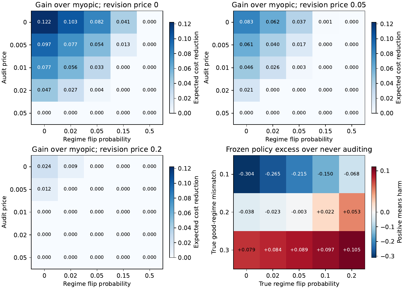
We retain every cell of a Cartesian sensitivity study at :
Of its 75 cells, 46 have zero improvement over repeated myopic control and 29 have strict improvement; the largest observed gain is . This finite grid neither defines a parameter distribution nor estimates a frequency of practical success. Prior sensitivity is stronger than a grid: the exact envelopes, comprising 83 and 76 retained pieces for coarse and fine incumbents, are exported over all .For misspecification we freeze the nominal history policy, then evaluate it under all 15 pairs and , leaving other parameters fixed. It is worse than the optimal never-audit comparator in seven cells. At its cost is , whereas never auditing and the true optimum both cost . The conservative bound here is , much larger than the observed regret; it should not be presented as a useful numerical guarantee at that perturbation size.
Negative controls and computational checks.
With uninformative audits and positive price, the optimum buys no audits; the reference model with also buys none. At , the next regime belief resets, but same-slot auditing can still help. For example, with and the original mismatch laws, auditing all eight slots costs , below the never-audit value . Thus “no regime persistence” does not imply “no information value.” Setting also removes installation inertia: choices then reduce to ordinary actions, a boundary of the representation interpretation.
The new scripts compare the policy-vector solver with a separate exact belief recursion in 300 small-horizon cases, check its line-envelope routine against direct minima at 1,844 critical points, and reproduce two exact values supplied by the independent specialist. A separate history-policy evaluator recovers every reported reference total and count. These checks supplement the printed induction and coupling proofs. Rational expectations remove Monte Carlo and discretization uncertainty; they do not remove model uncertainty, programming error or unverified implementation cost.
11.5 Prior art and what the extension contributes
Costly noisy HMM sensing and dynamic scheduling already appear in Krishnamurthy [6, Sections II–III]. Hidden-state tracking with repeated switching costs and hysteresis is explicit in Bayraktar and Ludkovski [2, Sections 1–2]. Reisinger and Tam [10, Sections 1–2] optimize observation timing and subsequent controls, including finite horizons. Their models differ in observation and action timing; those differences do not establish novelty for our combination. Together with the earlier acquisition references, they make a general priority claim untenable on this search alone.
The defensible gain over version one is an executable recurring-task contract, structural bounds, exact all-prior policies at declared horizons, an actual revisit witness and negative sensitivity evidence. It is meaningful mathematical generalization and synthetic validation, not realistic application validation or a new general POMDP theory. A calibrated benchmark requires an external task, defensible sensor and revision costs, and validation of the observation timing; none is supplied by renaming the latent regimes.
12 Research status and portfolio coordination
The original fixed-batch results survived this audit. Their simulation tables reproduce exactly, and the original delivered source, bibliography and code hashes agree with the earlier review closure. Those checks verify recorded artifacts and finite computations; neither previous nor current reviews are external human peer review or formal proof verification.
The two revisions turn part of the former prospectus into precise sequential and recurring-task models: an anytime sampling certificate, a cost-complete stopping problem, and repeated hidden-regime revision with exact policy envelopes and sensitivity bounds. The concentration, coupling and dynamic-programming methods remain established background; the worked contract and reproducible limits are the supported increment. Historical priority and standalone research novelty remain unestablished. The current prior-art audit is recorded with read depths and limitations, including relevant 2026 preprints; it is not exhaustive.
D02 boundary.
D02’s current continuation studies restricted noisy acquisition, including irreversible scout-and-commit permissions and paid stopping before a terminal prediction. This note instead pays to retain or replace an installed observable representation for a deployment block and, in Section 11, repeatedly during a common task stream. The unknown parameter here controls a feature’s usefulness, the objective is prior-averaged lifecycle cost, and no D02 minimax claim is imported. Merely selecting among D02’s noisy channels would not support a separate D04 novelty claim. Shared testing, concentration and Bellman lemmas should appear once in a combined volume. D06 concerns preservation under replacement, and D08 concerns solver verification; analogous value-of-learning mathematics should likewise not be counted twice.
What is now solved and what remains unresolved.
Section 11 solves a finite known-model case of repeated acquisition and revision while every deployment task continues. The complete parameter study and prior envelopes replace a single favorable example as the only evidence. It still assumes an immediately available independent audit, known transition and observation laws, a fixed two-candidate library, and uncharged planning resources. Unknown-model learning, delayed/selectively missing labels, task losses caused by audit delay, finite memory, and growing candidate languages remain unresolved. The observed sensitivity failures block any claim of robust practical superiority.
Interpretation and disposition.
The functional content is evidence-guided, priced discrimination. Supplied candidate maps and designer-specified objectives remain part of the contract. No claim about consciousness, intrinsic goals, or open-ended concept invention follows. Retain this as a technical methods companion to structural refinement and acquisition; seek a stronger coupled theorem and human specialist assessment before asserting research novelty or submission readiness.
References
- Sheeraz Ahmad and Angela Yu. Active sensing as bayes-optimal sequential decision making. In Proceedings of UAI, volume R11 of PMLR, pages 15–24, 2013. URL https://proceedings.mlr.press/r11/ahmad13a.html. Primary proceedings abstract inspected; no full proof audit claimed.
- Erhan Bayraktar and Michael Ludkovski. Sequential tracking of a hidden markov chain using point process observations. Stochastic Processes and their Applications, 119(6):1792–1822, 2009. URL https://arxiv.org/abs/0712.0413. Read arXiv version 2 of 22 May 2008; journal metadata checked separately.
- Norm Ferns, Prakash Panangaden, and Doina Precup. Metrics for finite Markov decision processes. In Proceedings of the Twentieth Conference on Uncertainty in Artificial Intelligence, pages 162–169, 2004. URL https://www.cs.mcgill.ca/~prakash/Pubs/Ferns_MetricsForMDPs.pdf.
- Wassily Hoeffding. Probability inequalities for sums of bounded random variables. Journal of the American Statistical Association, 58(301):13–30, 1963. doi: 10.1080/01621459.1963.10500830. URL https://www.cs.rpi.edu/academics/courses/spring06/random/hoefding.pdf.
- Steven R. Howard, Aaditya Ramdas, Jon McAuliffe, and Jasjeet Sekhon. Time-uniform, nonparametric, nonasymptotic confidence sequences. Annals of Statistics, 49(2):1055–1080, 2021. doi: 10.1214/20-AOS1991. URL https://arxiv.org/abs/1810.08240. Read archive version 9, revised 6 August 2022.
- Vikram Krishnamurthy. Algorithms for optimal scheduling and management of hidden markov model sensors. IEEE Transactions on Signal Processing, 50(6):1382–1397, 2002. URL https://ece.ubc.ca/~vikramk/Kri02.pdf. Primary author-hosted full text, relevant Sections II–III inspected.
- Lihong Li, Thomas J. Walsh, and Michael L. Littman. Towards a unified theory of state abstraction for MDPs. In International Symposium on Artificial Intelligence and Mathematics, 2006. URL https://ai.dmi.unibas.ch/research/reading_group/li-et-al-isaim2006.pdf.
- Omid Madani, Daniel J. Lizotte, and Russell Greiner. Active model selection. In Proceedings of UAI, pages 357–365, 2004. URL https://arxiv.org/abs/1207.4138. Original UAI 2004 paper; archive copy accessed 13 November 2026.
- Pierre-Yves Oudeyer, Frédéric Kaplan, and Verena V. Hafner. Intrinsic motivation systems for autonomous mental development. IEEE Transactions on Evolutionary Computation, 11(2):265–286, 2007. doi: 10.1109/TEVC.2006.890271. URL https://adapt.informatik.hu-berlin.de/pub/papers/ims.pdf.
- Christoph Reisinger and Jonathan Tam. Markov decision processes with observation costs: Framework and computation with a penalty scheme. arXiv:2201.07908v3, 2023. URL https://arxiv.org/html/2201.07908v3. Version dated 5 December 2023; relevant formulation inspected. Related journal DOI: 10.1287/moor.2023.0172.
- Reza Rezvan, Valter Schütz, Han Wu, Linus Aronsson, and Morteza Haghir Chehreghani. Active feature acquisition with incomplete training data. arXiv:2609.32325v1, 2026. URL https://arxiv.org/abs/2609.32325v1. Preprint, 26 September 2026; Sections 3–4 inspected on 13 November 2026.
- Hajin Shim, Sung Ju Hwang, and Eunho Yang. Joint active feature acquisition and classification with variable-size set encoding. In Advances in Neural Information Processing Systems, volume 31, 2018. URL https://proceedings.neurips.cc/paper/2018/hash/e5841df2166dd424a57127423d276bbe-Abstract.html. Primary proceedings abstract inspected for scope.
- Richard D. Smallwood and Edward J. Sondik. The optimal control of partially observable markov processes over a finite horizon. Operations Research, 21(5):1071–1088, 1973. doi: 10.1287/opre.21.5.1071. Publisher abstract and metadata inspected; finite-policy argument is supplied explicitly here.
- Brian Theory. Successive concept differentiation as observation refinement: Carrier splitting, interaction-core homology, and descent, 2026. URL https://www.b-theory.com/manuscripts-html/observation-refinement/. Referee-repair draft v0.5, 29 September 2026; site reading copy 3 with October 5 presentation clarifications. Accessed 13 November 2026.
- Edwin B. Wilson. Probable inference, the law of succession, and statistical inference. Journal of the American Statistical Association, 22(158):209–212, 1927. doi: 10.1080/01621459.1927.10502953. URL https://www.jstor.org/stable/2276774. Original printed p.209 score-interval formula visually checked in the full scanned article; nominal normal-score intervals used here, not exact coverage bounds. Accessed 13 November 2026.