When a Reference Goes Stale:
Self-Diagnosis under Shared Sensor Drift
AI-assisted research draft
13 November 2026
Classification: Technical note. Elementary finite-model results and a research prospectus; no priority claim. Internal AI review is distinct from external peer review.
Abstract
A calibrated observation mechanism need not remain calibrated. We study an actuator whose current reversal is to be diagnosed through two sensors sharing a drifting orientation bit. The environment is known, the target actuator bit is independently refreshed between tasks, and exact reference operations reveal the current sensor orientation at a stated price. Under these restrictive assumptions, routine observations provide no evidence about common orientation drift. We derive the exact diagnosis error as a function of reference age, a sharp maximum calibration interval for a prescribed mean-error bound at every deployed age, and the optimal long-run calibration cost over all history-dependent policies. Periodic calibration is sufficient because the observations relevant to scheduling are ancillary for the drifting orientation. We also derive an explicitly conditional extension for learning the drift rate and show why uncertain anchors, persistent targets, and health-informative sensor disagreement require different models. A separate coupled extension introduces hidden reference polarity and proves an exact reliability surcharge for a declared equal-drift maintenance model, including a certified regime with imperfect restoration and a counterexample to nominal-error reasoning. The results specialize elementary filtering and renewal arguments; unknown sensor polarity and anchor ambiguity already occur in the existing B-Theory corpus. The contribution is a fully reproducible contract for reference freshness, not a general theory of self-awareness or fault diagnosis.
1 Question, baseline, and contribution
Functional self-diagnosis requires evidence about a mechanism assigned to the agent. When the evidence channel changes, an apparent actuator fault may be a sensor-coordinate fault. An independently calibrated reference resolves that ambiguity only at the time and scope for which it is valid. The question here is therefore temporal: how often must an orientation reference be refreshed, and what does that requirement cost?
The actual baseline is stronger than a simple trusted-anchor model. Causal Self-Diagnosis with Noisy Tests, version 0.3 of 5 November 2026, explicitly includes unknown body and endpoint orientations, a simultaneous-flip ambiguity, and the insufficiency of a reference transmission without sensor anchoring, in Section 13.2 [1]. Its Section 14 also considers persistent preparation error and finite resources. Accordingly, neither an XOR ambiguity nor the need for independent orientation information is a new contribution here. Sensor Decisions under Unknown Dependence, version 0.2 of 9 November 2026, learns a stationary dependence law with known polarities and independent deployment episodes [2]. The changed assumption in this note is an orientation state that keeps evolving after calibration.
Blind sensor calibration has a substantial independent history. Balzano and Nowak study gain and offset identification from structured signal ensembles; their Section 4 identifies unavoidable scaling conventions [3]. Those linear models do not establish our binary age formula, and our intentionally unstructured fresh targets remove the redundancy on which their positive results rely. The mathematical machinery used below is elementary Bayesian decision theory, a two-state Markov calculation, and cycle-cost accounting. We do not assert that the resulting formulas are historically new.
Reference timing also belongs to the established literature on information freshness. Sun and Cyr explicitly give the symmetric binary Markov aging probability in Section III-B, equations (11)–(12), and optimize nonlinear age penalties in discrete time in Section IV-C, Theorems 3–4 [6]. Their channel model includes positive service times and a sampling-rate constraint; our reference is instantaneous and has a per-use charge. We therefore do not present our renewal formula as a direct corollary of their theorem without changing its timing assumptions. The substantive connection is that a diagnosis error can itself be an age penalty. The underlying binary aging law and optimization of freshness are established antecedents, not new results of this note.
The specific outputs are: an explicit observational symmetry; an exact reference-age risk; an optimal renewal characterization under a stated information restriction; and failure cases identifying the assumptions that would have to change in a more realistic experiment. They support a technical addendum to the diagnostic research family. They do not yet justify a separate flagship research paper.
2 Operational contract
Time is indexed by deployment tasks . All logarithms in statistical bounds are natural. The physical and information variables are as follows.
is the actuator reversal on task . The sequence is independent and fair, and independent of all sensor variables. This is a supplied task ensemble, not a claim about the typical persistence of faults.
is a common sensor-orientation state. Initially it is fair, and , where the are independent Bernoulli variables. Initially is known and .
The environment contributes a known zero reversal. A command produces the binary physical output . The two sensors return , .
The are independent Bernoulli variables, , independent over tasks and of everything else. Both sensors share ; independent readout noise does not imply independent calibration errors.
Before issuing the current command or seeing its readings, the controller may pay for an exact anchor . This operation neither changes nor advances the task clock. Its physical realization is an assumption.
The controller then chooses , receives both readings, and reports . The loss is . The next orientation transition happens only after the report.
Policies may depend on the complete retained action, reading, and anchor record, and on independent private coins. They cannot see , without anchoring, or future flips. Computation and record storage are unpriced; this note makes no computational-efficiency claim. The comparison is among policies with the same prior, known parameters, two mandatory readings per task, and report timing. A known-current-orientation oracle has a strictly stronger information interface and is labeled accordingly.
The target is the current actuator bit, not the original actuator state. There is no repair action in the core model. Calibrating the readout is not repairing the actuator. The self/world boundary and reference accuracy are assigned by the model; neither is inferred from a correlation.
Write and . The command cancels, so arbitrary adaptive commands cannot improve this task. If the last anchor occurred at , define its age as . A task on which an anchor is purchased has age zero.
3 Ambiguity and what the second sensor can establish
Proposition 3.1 (Common-orientation ambiguity; elementary specialization). Without any anchored orientation, the complete routine transcript has the same law under and . Under the supplied fair prior, every routine-only actuator estimate has Bayes error at least . The pair of routine readings on each task is independent of the entire orientation trajectory, even though it carries information about .
Proof. Flipping both coordinates leaves unchanged and leaves the orientation-flip increments unchanged. The transition and observation kernels, and the prior, are invariant. Equal past transcripts induce identical action distributions; induction therefore preserves the equality for adaptive randomized policies. For any fixed orientation trajectory, the fresh bits are independent fair bits. Integrating the known readout-noise channel yields a routine-transcript distribution independent of that trajectory, including adaptive commands after their known offsets are removed. Consequently remains fair without an anchor. Given any routine observations, is fair, proving the Bayes claim. ◻
This proposition is included to expose a contract, not to claim a new gauge principle. It is directly analogous to the already stated orientation ambiguity in B07. It also explains an empirical trap: agreement between sensors can establish a common reading while giving no evidence that their common coordinate system is correct.
With a fresh exact anchor, two equally accurate independent sensors have Bayes error . To check this, on agreement the preferred bit is their common value; on disagreement the posterior is tied. Thus the error is (1) Two readings do change conditional confidence: agreement error is (2) Therefore the equality of average error with one sensor is not equivalence of the experiments for every decision problem. An odd number of independent readings would reduce by ordinary majority voting, without removing uncertainty about .
4 Exact reference aging
Theorem 4.1 (Age-dependent diagnosis risk; proved here as an elementary calculation). Under Section 2, the minimum expected classification error on a task whose latest exact anchor has age is (3) The statement holds conditional on any admissible past that schedules the task at that age. In particular, a history-triggered calibration rule cannot use previous routine data to obtain a lower risk at the same age.
Proof. The parity has sign expectation
Hence its probability of one is . Future flips are independent of the most recent anchor value and of all routine data. In particular, deciding not to anchor on intervening tasks does not select unusually stable orientations: the decision uses only information independent of those flips. The event defining a given age may depend on earlier anchor values, but the most recent anchor restarts the independent flip process.For any current reading pair , let . Its sign specifies the optimal estimate of . Mixing over the orientation parity multiplies this posterior contrast by , up to the known sign of . Since , the sign does not reverse. Conditional error is . Averaging and using proves (3). This proof also covers disagreement, where . ◻
Corollary 4.2 (Maximum interval for a mean-error requirement). If , a policy that must have mean classification error at most at every deployed age can use only ages (4) Periodic calibration every tasks satisfies the requirement exactly when .
Proof. The risk requirement is equivalent to . Taking logarithms reverses the inequality because . The ages in a length- cycle are and the risk increases with age. ◻
This is a guarantee about average error over the two readings and the supplied target ensemble. It is not a bound on every realized posterior error: disagreement has posterior error even at age zero. When the fixed observation interface is insufficient. When no calibration is required for this criterion.
5 Optimal calibration timing
For an integer , periodic calibration has average cost (5) Never calibrating has error and zero calibration cost. Let (6)
For a permitted policy , write if it buys an anchor at task and otherwise. Its expected upper-average loss is
The expectation is taken before the upper limit. Replacing the upper limit by a lower limit of the expected averages gives the same optimal value: the proof gives a finite-horizon lower bound for every policy and an attaining policy whose expected averages converge.Theorem 5.1 (No benefit from ancillary scheduling). For the infimum of over all policies in Section 2 equals . If , some finite renewal period attains the value. If , never calibrating is optimal.
Proof. At each task, conditioning on the scheduler’s available information before the current readings gives the minimum age cost in Theorem 4.1. Every reporting rule has conditional classification risk at least that minimum, with equality for a Bayes report. By the tower property, expected total classification cost is therefore at least the expectation of the sum of these age costs. This does not condition on the entire realized future schedule, which could contain information from future anchors. For a finite run, group the age costs pathwise into consecutive calibration segments. Every segment of length , including the final truncated one, has cost . Any initial segment before the first anchor has cost . The inequality holds for every sequence of segment lengths, hence also after expectation over randomized scheduling. Every finite-horizon expected average is therefore at least , even if a policy has no limiting average.
A fixed finite period attains by direct summation, and the never-anchor policy attains . Put . If , equation (5) gives for every finite . If , then for sufficiently large , , so some . Since , the infimum below must be attained in a finite set of periods. This supplies an attaining policy. ◻
The cycle argument is a specialization of ordinary average-cost control, not a general claim that periodic recalibration is best. It relies on all scheduler observations being uninformative about the unobserved orientation increments. A sensor-health alarm, a persistent actuator target, unequal orientation-dependent noise, or an anchor taking time invalidates that premise.
At , a single exact calibration followed by no further anchors gives limiting risk at any finite initial charge. The formula dividing by must be read by continuity, but “never anchor” and “anchor once” remain different policies. At , only age zero benefits: . At the readings carry no actuator information even with calibration. At anchoring every task is optimal. These cases make clear why a frequency statement needs its parameter domain.
6 Learning a drift rate and deciding when to abstain
6.1 A finite training contract
Suppose is unknown but constant. For an integer and , perform exact reference observations at consecutive task boundaries, yielding observed independent flip indicators. With their mean , set (7) Hoeffding’s one-sided bound [4, Theorem 2] implies . For fixed , is increasing in on . When , a frozen period satisfying Corollary 4.2 at therefore meets the mean-error requirement at every deployed age on that one good-training event. At the clipping boundary , the logarithmic formula is not used: if , choose period one, since age zero has risk and every positive age has risk at the upper-bound model. If , the fixed observation interface cannot meet the requirement. The training anchors cost ; their cost is not hidden in deployment performance. This is a standard concentration wrapper, not an optimal sample-complexity theorem.
The per-task mean guarantee is conditional on the parameter being covered. It does not say that no deployment error occurs. A finite number of correct calibrations cannot rule out later changes in , arbitrary adversarial polarity drift, or a defective reference. Time-varying rate estimation and sparse-anchor experimental design remain separate problems.
6.2 Abstention uses conditional risk
Suppose an abstention costs and an incorrect report costs one. For the symmetric sensor pair, disagreement must be rejected because its conditional error is . On agreement the conditional error at age is (8) The optimal terminal rule accepts agreement exactly when . It is incorrect to threshold the unconditional and claim a per-report guarantee. The coverage on an accepted age is ; it is zero at rejected ages. Optimizing calibration jointly with selective coverage is an extension with a new cycle reward, not a consequence of (5) without recomputation.
Abstention from attribution need not prohibit action. If all currently compatible explanations permit the same shutdown or reference-restoration action, it can be selected without deciding which actuator label is true. The general common-action principle is already explicit in B07, Section 7.1; no new theorem is claimed for it here.
7 Reproducible checks and worked example
The supplied code/reproduce.py uses rational arithmetic
to enumerate the two sensor noises, current target, and orientation
parity. It checks (3) at four values each of
and
and ages zero through twelve: 208 checks. It separately enumerates all
binary calibration schedules for horizons one through eight and compares
them with an age-state Bellman recurrence. These checks test the timing
convention and implementation; the proofs establish the unlimited-age
and all-policy statements.
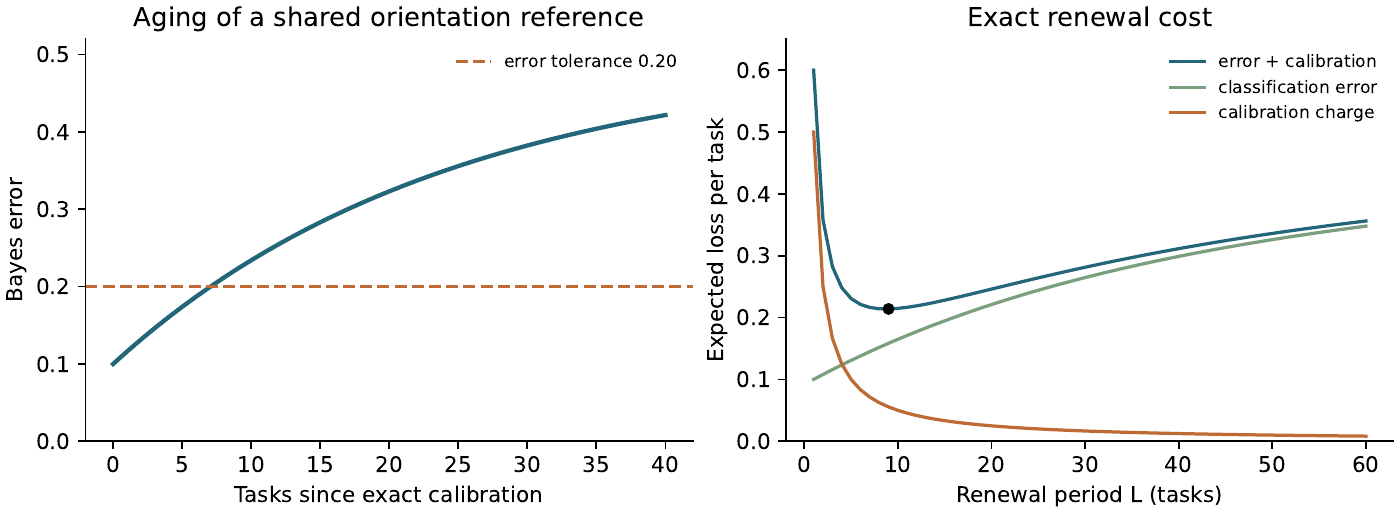
For , , and , equation (3) gives , , and . A mean-error requirement of permits maximum age seven and hence period at most eight. The plotted renewal curve and tabulated values are evaluated from exact rational expressions before conversion to decimal. A finite search through period 200 is identified as such in the output; its minimum is corroborative, not a substitute for the global cycle theorem.
8 Failure boundaries and unresolved investigations
A fixed actuator is a different problem.
If forever and a noiseless anchored measurement identifies it once, later sensor drift does not erase the retained actuator label. Reusing formula (3) would incorrectly predict a need to relearn a bit already known. Fresh independent targets are the reason routine histories cannot track here. A persistent but changing actuator requires joint filtering of actuator and sensor changes.
An imperfect reference is not exact renewal.
If the latest anchor has independent orientation error , a decoder using only that anchor has risk . This follows by multiplying sign correlations. It is not the full-history optimum: earlier imperfect anchors can provide additional information. If a reference shares an unknown permanent orientation with the sensors, the initial symmetry persists and absolute diagnosis may remain impossible.
Repetition does not manufacture independence.
Reusing one readout-noise bit gives one corrupted observation, irrespective of the number of times it is read. Repeated common-mode observations cannot replace an independent reference. Conversely, structured task distributions can make blind calibration possible, as in the linear signal assumptions of Balzano and Nowak [3]; the impossibility here is not universal.
General joint drift is unresolved.
A useful next model has persistent , separate sensor orientation chains, and imperfect calibrations of known reliability. Its posterior is a finite-state hidden Markov filter. One should compare exact finite-horizon belief-state control with periodic and alarm-triggered calibration under identical readout costs. No optimality theorem for those extensions is asserted. A second question is whether a lower bound on calibration expenditure survives a robust class of unknown flip rates, with the physical reference itself degrading. These are explicit research proposals.
10 Imperfect restoration: a certified range and a failure case
The previous theorem supplies perfect symmetry breaking. To test that assumption, replace only the restoration operation: it sets to an unobserved fresh , , independent of the old state and all other randomness. It then rereads . The controller knows , but not whether restoration succeeded. A single such operation is available per augmented probe; it has the same surcharge and timing as before. Physical service lives remain observed. This models a calibrated stochastic reset, not arbitrary imperfect repair or an empirically certified mechanism.
Here reliability is required conditional on the entire report-time record, including the selected action, the restored reference readout, and the current routine readout. This strengthens any interpretation that averages over the restored reference result. The fresh fair target makes the routine readout independent of orientation, so it does not alter the orientation posterior. Put . For a pre-restoration orientation contrast and restored sign , Bayes’ rule gives (11) Both denominators are positive. The exact conditional diagnosis error is . If one ignores the old record, the reference has average error ; that is not a bound on each conditional error after combining the record with a conflicting readout.
Proposition 10.1 (Reachable failure of nominal-error reasoning). Take , initially fair orientation, and the four-action restored-probe cycle. After a first restored sign , four successive transitions, and an opposite restored sign, the report-time Bayes error is despite nominal reset error .
Proof. The first posterior contrast is . Each multiplies it by . Before the next reset it is . Substitution of in (11) gives the stated error. All events have strictly positive probability: the initial sign has probability , each no-change event has probability , and the final conflicting sign has probability . Physical feasibility can be ensured with . Thus this is a reachable failure within the priced cyclic interface, not merely an arbitrary prior. ◻
Theorem 10.2 (A certified imperfect-restoration regime). Retain equal drift and define If and , the imperfect-restoration model has a nonempty reliable recurrent kernel exactly when . If , that kernel is empty at every resource level. No classification of the intermediate range is asserted.
Proof. In the four-action cycle, four hidden transitions separate consecutive restored probes. Their contrast multipliers are either or zero, so the pre-restoration contrast satisfies , independently of prior reset outcomes. Before the first probe the contrast is zero under the supplied fair initialization. When , formula (11) gives
The lower bound follows by choosing the conflicting sign and maximizing up to ; differentiation of gives . Thus every possible report in the affordable restored-probe cycle meets the requirement. Resource sufficiency is exactly the previous cycle argument.For necessity, a tick with still erases the old contrast. An ordinary probe then has error ; an imperfectly restored probe has error exactly for either restored outcome. For any , every allowed probe on an all-change run must therefore pay restoration. The finite-run resource argument of Theorem 9.2 gives the same necessary bound . If , no probe on such a run is permitted at all. Four consecutive all-change ticks have positive probability and force a probe by the monitor, contradicting infinite feasibility regardless of resources. ◻
For and , , and . Thus admits the sharp resource threshold even though restoration is not perfect. The value is a conservative sufficient bound; its attainability or optimality over all belief policies is not claimed. The theorem does not prove feasibility or infeasibility throughout , nor when .
Validation and what remains assumed.
The supplied script enumerates hidden-state probabilities independently of the posterior formula, checks the counterexample exactly, and expands all observation branches of a finite prefix of the restored-probe cycle. This is synthetic model validation, not device data. The infinite-horizon assertion rests on the uniform bound and resource proof. The stochastic reset remains an externally calibrated, independent channel; correlated repair faults, uncertain , unequal drift and time-consuming restoration are unresolved. D05’s separate paid exact-reference action consumes a full tick and obeys a different theorem. Neither its threshold nor the present instantaneous-surcharge threshold transfers across those timing contracts.
11 Being, Becoming, The MIND, and publication status
The operational capability studied here is recognizing the limited lifetime of evidence used for self-attribution. “Being” refers to the presently available calibrated diagnostic interface; “Becoming” includes changes in that interface and its restoration; “The MIND” refers to the controller’s actionable record of reference age and uncertainty. Those interpretations are not additional mathematical results, and no inference to phenomenal consciousness, personal identity, or a uniquely natural self/world boundary follows.
D08 concerns computation quality; this note concerns physical evidence validity. D05 can incorporate reference age while charging the resources needed for recalibration. The preferred publication role is a diagnostic addendum or a section of an integrated D03/D05 study. General imperfect-reference control, device validation, and external priority review remain open; Section 9 solves only its stated equal-drift special case. The arguments have not undergone formal verification or external peer review.
References
- B-Theory research programme. Causal self-diagnosis with noisy tests: Observation laws, irreversible access, and task recovery, 2026. URL https://www.b-theory.com/read-online/causal-self-diagnosis/. Version 0.3, 5 November 2026. Byline: Research development draft prepared for Brian Theory; AI-assisted derivation, computation, and independent internal review. Submission authorship undecided.
- B-Theory research programme. Sensor decisions under unknown dependence: Interval frontiers and paid calibration, 2026. URL https://www.b-theory.com/manuscripts-html/sensor-paid-calibration/. Technical addendum, version 0.2, 9 November 2026; not externally peer reviewed.
- Laura Balzano and Robert Nowak. Blind calibration of sensor networks. In Proceedings of the 6th International Conference on Information Processing in Sensor Networks, pages 79–88, 2007. doi: 10.1145/1236360.1236372. URL https://nowak.ece.wisc.edu/BalzanoNowakIPSN07.pdf.
- Wassily Hoeffding. Probability inequalities for sums of bounded random variables. Journal of the American Statistical Association, 58(301):13–30, 1963. doi: 10.1080/01621459.1963.10500830. URL https://www.cs.rpi.edu/academics/courses/spring06/random/hoefding.pdf.
- Jiping Luo, George Stamatakis, Osvaldo Simeone, and Nikolaos Pappas. Remote state estimation over a wearing channel: Information freshness vs. channel aging, 2026. URL https://arxiv.org/html/2501.17473v2. arXiv:2501.17473v2, 14 May 2026.
- Yin Sun and Benjamin Cyr. Sampling for data freshness optimization: Non-linear age functions. Journal of Communications and Networks, 21(3):204–219, 2019. doi: 10.1109/JCN.2019.000035. URL https://arxiv.org/abs/1812.07241. Relevant technical statements read in arXiv:1812.07241v4, 3 May 2019; journal metadata checked separately.
- Chiel van Oosterom, Lisa M. Maillart, and Jeffrey P. Kharoufeh. Optimal maintenance policies for a safety-critical system and its deteriorating sensor. Naval Research Logistics, 64(5):399–417, 2017. doi: 10.1002/nav.21763. Accepted manuscript dated 3 September 2017, obtained from Eindhoven University repository; full text including appendix read in second audit.