Driven Binary Memory with Failure Detection
and Fuelled Repair
AI-assisted research draft
November 13, 2026
D10 — Revised technical note with an explicit maintenance network. The physical model is a specialization of established information thermodynamics. The closed forms and design optimization are elementary derivations, not a claim of a new universal thermodynamic law. Internal review is not external peer review.
Abstract
What does it cost to keep a finite physical memory informative about a changing signal? We analyze a binary memory driven by a symmetric two-state signal, with a specified energy gap, thermal transition rates, and externally supplied work. The stationary tracking error, future prediction risk, work input, heat output and information-flow rate are derived explicitly. With a fixed maximum response rate, we obtain the exact minimum stationary power within this two-parameter device family for a prescribed error tolerance. A finite energy-gap restoration protocol prices a scheduled change. We then add physical health and detector states, reversible repair reactions and a maintained chemical fuel source. A symmetry theorem shows why one memory snapshot cannot diagnose health, and a two-channel counterexample exposes dissipation hidden by coarse repair rates. The baseline formulas are checked against the full four-state master equation and numerical integration; the extension is checked with independently assembled sixteen-state and eight-state generators. This model does not identify a universal price of learning, include all costs of the signal generator or controller, or solve unknown-reference recalibration. The extended maintenance subsystem has autonomous internal kinetics, but finite chemical fuel, microscopic hardware validation and optimal feedback remain open; an explicit finite battery and a common-budget controller menu are analyzed separately. The result is a small physically grounded bridge from the portfolio’s abstract resource contracts to an implementation-specific design calculation.
1 Question and relation to established work
D01 separates target uncertainty from memory entropy; D05 assigns resources to maintaining diagnostic capacity. Neither accounting system alone identifies physical work or heat. Existing MIND constructions explicitly separate Boolean operators, stochastic channels and physical implementations [1, Section 1]. The present question is narrower: for a declared thermal memory and externally changing signal, what stationary power realizes a given prediction capability?
The relevant baseline is mature. Horowitz and Esposito formulate bipartite Markov thermodynamics and split mutual-information flow across subsystems [8, Sections II–III, equations (1)–(12)]. Barato, Hartich and Seifert analyze cellular sensing, including a four-state model and bounds connecting its learning rate and entropy production [3, Sections 2–4]. More precisely, the four-state generator is exactly the toy model of Barato, Hartich and Seifert [2, Section II, Fig. 1, equations (3)–(4)] under and . Their entropy-production formula becomes (10). The present work does not introduce that generator or dissipation formula. We retain its rates in a response-budget parametrization and solve a constrained design problem; priority for that elementary optimization is not established.
Still and colleagues consider a system driven without feedback, with alternating signal-change and relaxation steps; their dissipation–prediction identity uses a specific nonequilibrium free-energy convention [13, equations (1), (8), (14)–(18)]. We do not substitute our stationary continuous-time quantities into that discrete-step identity. Instead all balances below are reconstructed directly. Kolchinsky and Wolpert define semantic information through explicit scrambling interventions and a chosen viability functional [9, Sections 3–5]. Our prediction risk is not their viability functional, and no semantic-information or autonomy theorem is inferred merely from a correlation.
2 Physical and operational contract
2.1 States, rates, and energy bookkeeping
The external signal flips at rate , independently of the memory. The physical memory has energy (1) It is coupled to a single bath at temperature . Set and (2) where is the sum of the two conditional response rates. Signal transitions are at rate . Simultaneous jumps have probability zero. Time is continuous; rates have units of inverse time.
The memory transition-rate ratio is , so memory jumps satisfy local detailed balance for the stated energy gap. A signal jump changes the energy landscape. Its energy change is supplied as work by an external modulation mechanism, not as heat from the memory bath. Thus one must not interpret both coordinate flips as passive thermal jumps with respect to . If all four transitions were passive in one bath, the signal rates would generally depend on and the contract would change.
Let denote heat delivered to the bath, positive when the memory loses energy in a thermal jump; denotes work supplied by signal modulation or a scheduled change of . The first law is (3) This boundary includes the memory’s energy and the work delivered to it. The signal generator, clock, feedback electronics, fabrication, sensing readout and controller are not given microscopic dynamics. Their additional costs are outside the reported power. An ideal externally driven experiment is a permissible model, but is not a self-maintaining autonomous organism.
2.2 Information, policies, and target
The observer may read the current at a declared time and predict for a fixed horizon without future readouts. Only the current memory is available, not the whole memory trajectory or the signal itself. For this experiment, readout is ideal and its apparatus cost is excluded as above. The loss is prediction error probability. Parameters are known; no estimation phase or unknown sensor orientation is hidden in the calculation.
In the design problem, the admissible devices have one fixed and one fixed finite over the evaluation interval. They are compared in stationarity under the same , same readout rights and same target. Adaptive driving, extra memory states, time-dependent steady protocols, trajectory decoding and different reservoirs are outside this policy class. The finite restoration protocol later is a separate nonstationary experiment, not a competitor smuggled into this optimum.
Information is measured in nats here. Multiplication by converts a Shannon entropy of physical states to the corresponding coarse-grained entropy contribution; multiplication by converts a dimensionless free-energy expression to energy under the stated physical assumptions. Internal degeneracies of either logical state are assumed equal and absorbed into . Different degeneracies would change the free-energy gap and rates.
3 Stationary tracking and future prediction
Let . Signal flips exchange match and mismatch. Memory transitions create mismatch at rate from a match and remove it at rate from a mismatch. Consequently (4)
Proposition 3.1 (Stationary error and response). For and , the four-state chain has a unique stationary law, (5) For an arbitrary initial mismatch probability, (6)
Proof. All four states communicate since the signal flips and both memory directions have positive rates, so a finite irreducible chain has a unique stationary law. The generator is invariant under . Uniqueness therefore forces the two match probabilities to agree and the two mismatch probabilities to agree. Equation (4) fixes their sum to the displayed ; substitution verifies every balance equation. Solving the scalar linear differential equation gives (6) without requiring an initially symmetric joint law. ◻
The stationary marginal of either bit is uniform. Thus (7) Meanwhile for every parameter value. Memory-state entropy alone cannot measure sensing quality in this example.
Proposition 3.2 (Prediction at a fixed horizon). Under the stationary law, the Bayes predictor from for is (with a tie at ), and its error is (8)
Proof. The number of future signal flips is Poisson with mean , independent of the current pair. Its parity is odd with probability . Conditional on the current memory, future mismatch therefore has probability , giving the formula. This is at most because , so predicting the observed bit is Bayes optimal. No computation on the same single bit can beat its posterior risk. ◻
Tracking the current signal and predicting a distant signal are different tasks. Increasing pushes the error toward even with an informative current memory. None of the comparisons in the frontier below changes this horizon.
4 Work, heat, and information flow
The aggregate rate of thermally correcting a mismatch minus creating one is (9) A correction releases ; a thermal error absorbs it. A signal flip starting from a match raises the energy by , while one starting from a mismatch lowers it by . Therefore stationarity gives (10) Here has units of inverse time, or nats per unit time in the entropy balance. is the bath entropy current. It also equals the stationary Markov entropy-production rate of this effective four-state description, obtained by summing each undirected edge current times its forward/backward probability-flux log ratio. This does not assert that the omitted modulation apparatus has zero entropy production.
Proposition 4.1 (Information-flow specialization). The memory-transition contribution to the stationary mutual-information derivative is (11) The signal contribution is , and the total time derivative of mutual information is zero in stationarity.
Proof. At the stationary symmetric law, . Considering only memory jumps, , so their contribution to is . Signal jumps give , with the opposite contribution. Since
and , both logarithms are nonnegative and . Multiplication by proves the bound. At both quantities are zero. ◻This is a direct specialization of established bipartite information-flow results [8, 3], not a new inequality. A learning rate, a trajectory mutual-information rate, the instantaneous mutual information, and its total time derivative are different quantities. The last is zero here even while information is continually renewed.
5 Exact stationary frontier within the declared device family
We now optimize over the physical parameters instead of reporting one favorable device. Fix and an allowed current error . Write (12) This is an infimum reached only at infinite energy gap when ; it is not a finite-parameter device.
Proposition 5.1 (Family-specific minimum power). If , the minimum stationary work rate over the admissible devices satisfying is (13) It is attained at and . No finite-gap admissible device attains . A tolerance can be met with and zero stationary power.
Proof. Solving (5) for at a desired error gives (14) Positivity of is equivalent to , proving the feasibility condition and the unattained lower boundary. At fixed feasible , increasing increases and decreases . The other factor is fixed, so power is minimized at .
It remains to check that a stricter error than requested cannot lower power. At fixed , both positive factors and strictly decrease as increases in . Their product therefore strictly decreases. The optimum subject to is at . Substitution into (10) proves the expression and its attainability by finite . At , and provide the zero-power case. ◻
For a future error tolerance at fixed , use
in Proposition 5.1, checking feasibility first. The optimal value diverges as the required approaches from above. Unlimited response speed would change the admissible family: as , the frontier approaches . This is the information-flow lower envelope for this family, not evidence that an arbitrarily fast physical apparatus is free.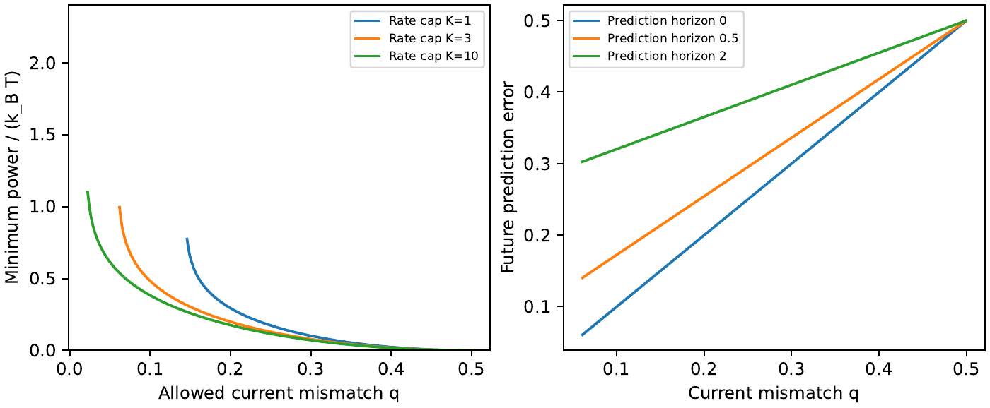
6 A physically accounted restoration protocol
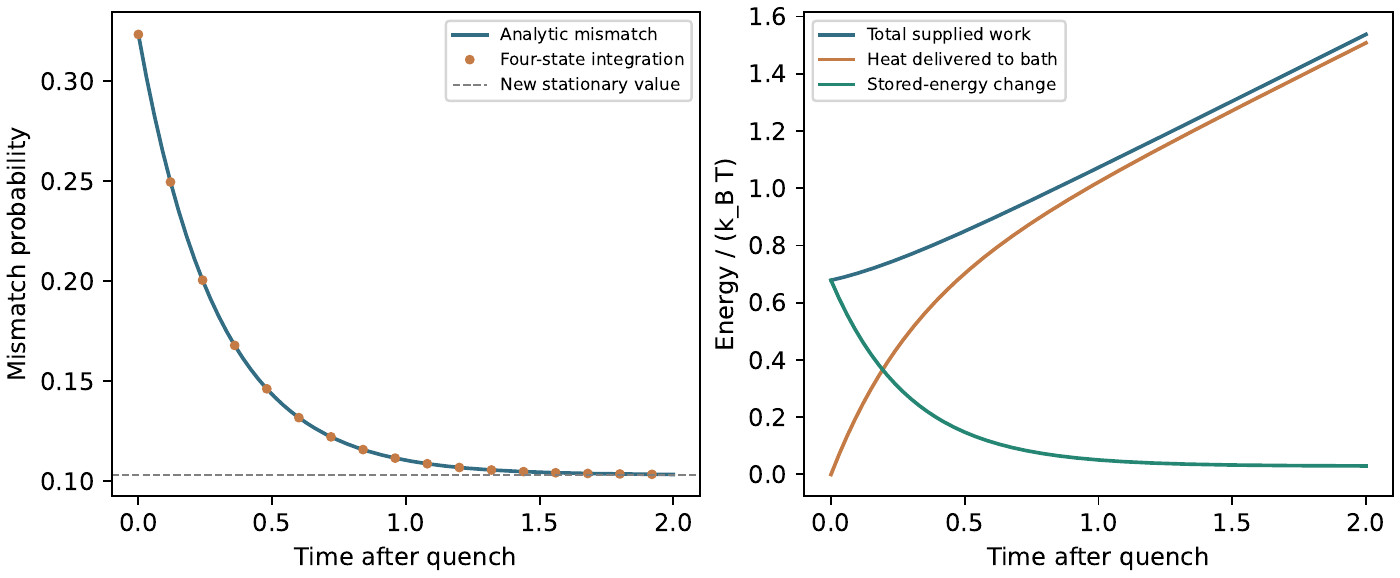
An abstract cost for “recalibration” does not specify where energy goes. As a minimal physically priced modification, suppose a known weakened coupling with gap is restored at time zero to a stronger , while remain fixed. The change is a scheduled, instantaneous Hamiltonian quench: no state changes during the switch. The pre-quench distribution is stationary with error ; afterwards the target stationary error is and the new thermal parameter is .
This is restoring a known coupling energy. It is not inferring an unknown calibration, discovering a broken reference, manufacturing a new component, or autonomously deciding when to repair. The control schedule and switch mechanism are assumptions. Within those assumptions, the following accounting is exact.
Proposition 6.1 (Finite restoration balance). Let and Then the quench work, subsequent signal-driving work and subsequent heat output are (15)(16)(17) They satisfy (18)
Proof. The quench changes energy only on the mismatch states, of total probability , giving the first expression. At later times, the work rate is and the heat rate is , by the same state-transition accounting as before. Since , integration gives the displayed formulas. Subtracting the heat rate from the work rate gives by (4); integrating and adding the quench establishes the first law. ◻
For , , and in units , the mismatch changes from toward . The quench supplies about energy units. At time two, total supplied work is about , heat output about , and the difference remains stored energy. These values come from the included computation and obey the finite balance, not only a stationary equality.
7 A physical detector and fuelled repair network
The four-state frontier concerns a fixed device, not maintenance. We now give a separate, time-homogeneous finite-state model in which failure, detection and repair are transitions. Its thermodynamic laws are standard channel-resolved Markov accounting [5, Section II, equations (3)–(19)]; the contribution is a specified, reproducible maintenance example with explicit limitations.
7.1 States and local detailed balance
Let . The health state denotes a weak memory and a strong memory; is a physical alarm state. Define (19) All states have equal internal degeneracy. There is a common bath at , a maintained chemical free-energy difference , and the original external signal. For a coordinate flip , put . Choose and . The directed rates are (20) The alarm gate is . On a health edge it multiplies both reaction directions, since is unchanged. When the gate is closed, both fuel rates vanish; these absent edges contribute nothing to entropy production. Thermal health transitions remain possible. The controller is the physical detector conformation and its assumed catalytic gating; no observer supplies as an error-free input. No scheduled clock or digital reset is required by this model.
A fuel-channel health transition consumes chemical free energy ; its reverse returns . Thermal jumps receive no work. Every non-signal channel satisfies (21) where on fuel edges and zero otherwise. Here denotes energy per event, not a transition rate. On signal edges is external work, the forward and reverse rates are equal, and no bath heat is assigned. Thus signal symmetry is not being asserted as passive thermal detailed balance.
The health transition energy is (22) The detector therefore acts back on health. Omitting its interaction energy from repair would violate the declared local detailed balance. Likewise a constant repair/reverse ratio cannot implement a fixed when varies. The reverse chemical reaction cannot simply be deleted at finite affinity. Here “repair” means conversion to the designated strong conformation, not perfect restoration or replacement of a damaged material.
This is a mesoscopic thermodynamic realization, not a fabricated controller or atomistic derivation. Attempt rates and catalytic barriers are assumed fixed hardware. The maintenance subsystem is autonomous in the sense of time-independent internal kinetics, while the whole device remains externally powered: the signal source, maintenance of the chemical reservoirs, construction, readout apparatus and eventual replacement of the controller itself remain outside the boundary. A maintained is not a finite fuel tank.
7.2 Channel-resolved energy and entropy balances
Let be the unique stationary law; positivity of the thermal coordinate rates and gives irreducibility even if . Sum each unordered state pair once for each available reaction channel , and orient it arbitrarily. Write
Absent fuel pairs have current zero. Define (23) For signal edges the heat term is zero. Signs of individual channel heat flows need not be positive.Proposition 7.1 (Stationary maintenance balance). For the finite network above, (24) Consequently the fuel current and signal work, not an abstract count of detected failures, determine the stationary energy bill within this boundary.
Proof. Each transition obeys . Summing event rates gives the first law; stationarity sets . In , the terms sum to the stationary Shannon entropy derivative, zero. The remaining log-rate terms equal by (21); they vanish on the symmetric signal edges. This proves the equality. Each summand for positive forward and backward probability fluxes is nonnegative. The assertion follows without an information-to-energy conversion postulate. ◻
7.3 What the memory and alarm can diagnose
A predictor is not automatically a fault detector. The following is an elementary symmetry consequence, related conceptually to D03’s observation ambiguities but using a different interface: one physical snapshot rather than a fresh-target observation history.
Proposition 7.2 (Snapshot blindness). For any irreducible generator on invariant under , its stationary law satisfies In particular . The minimum probability of incorrectly classifying health from alone is , identical to using no observation. All rates in (20) obey this symmetry.
Proof. Uniqueness forces the stationary law to be invariant under the permutation. Summing over gives equal probabilities for and at every fixed , proving independence. Every conditional health posterior given therefore equals its prior; a majority-prior decision minimizes zero-one loss. ◻
The proposition does not cover a memory trajectory, a simultaneous readout of and , or a nonstationary initialization. Waiting times and disagreements can reveal health. Instantaneous and trajectory information are different quantities [7, Section II]. For a single alarm readout the Bayes health risk instead is
Positive need not strictly reduce this particular risk: posteriors can move without crossing the decision threshold. The gate is a specified catalytic response, not a claimed Bayes-optimal maintenance policy.For prediction using only , symmetry gives a symmetric marginal. Write its mismatch probability as ; it is obtained from the full joint stationary law, not by substituting an averaged into Proposition 3.1. Since future signal flips remain independent, the Bayes error at horizon is (25) This follows by choosing or its complement according to the sign of . It does not require a general claim that every feedback design has .
7.4 A finite calculation and an adverse detector example
In units , take , , , , , , , . The full 16-state generator gives
The detector-channel heat output is ; this is a channel flow, not a separately identified minimum detection cost. Aggregating parallel health reactions before calculating entropy production gives only , missing dissipation.The joint law with rows and columns is
Although nats, the Bayes classifier always reports healthy, so , equal to the prior-only risk. Reporting has larger error . The false-alarm probability given healthy is , and the missed-alarm probability given weak is . This example prevents equating correlation, detection accuracy and useful control.In the recorded sensitivity grid, changing only to at gives , below the prior-only risk ; the detector can be informative for classification. This is a different physical device with altered interaction and backaction, not a free improvement. The code also evaluates disabling the fuel channel and opening it for both detector states. Those settings trade prediction against work; they are neither a global optimization nor comparisons at matched risk. No advantage over the original frontier is claimed because the state space and rate contract have changed.
9 Finite energy storage and a matched maintenance contract
A maintained chemical potential is an inexhaustible external resource. To expose this boundary, replace the chemical channel by a finite battery with equally degenerate levels and total energy
This is an ideal finite energy ladder, not a finite well-mixed chemical reservoir. Finite chemical reservoirs and explicit replenishment already have substantial antecedents [6, Section II]; conservation laws in chemical thermodynamics are established [10]. A recent preprint derives open chemical-network dynamics and thermodynamics from closed systems under time-scale and abundance separation [11]; the present ladder example establishes no such limit. The construction below supplies a bounded maintenance example, not priority for finite-reservoir thermodynamics.For , pair with . Write and set
Both rates belong to that same pair. A forward repair consumes one level, its reverse restores one. No transition crosses a battery boundary; all other original thermal channels leave unchanged. Signal jumps still do external work. Local detailed balance now holds against the total energy change , without an external chemical-work term. The forward and reverse updates change two coordinates together, so a single-coordinate multipartite information-flow theorem must not be applied without regrouping health and battery.Proposition 9.1 (Finite battery accounting). Let count forward and reverse battery-channel events. Pathwise, The mean energy balance for the enlarged device is whereas the memory/controller boundary alone satisfies In every stationary law the net battery current is zero. Moreover, as .
Proof. Only battery-channel events change , by respectively minus or plus one. Summing these increments gives the pathwise identity and bound. For each such event the battery-energy loss cancels work delivered to the device; summing all event energies gives the first laws. Stationarity implies ; the long-time conclusion also follows directly from boundedness, without irreducibility. ◻
denotes net energy drawn from the ladder, not automatically reversible work or free-energy depletion. The battery distribution can gain entropy and correlate with the controller; extractable-work accounting would additionally require those terms. The budget below constrains this explicit energy statistic.
The proposition does not bound the gross number of repairs by . A thermal health failure followed by repair discharges the battery; a reverse battery event followed by thermal recovery charges it. Thus is generally not absorbing, and the externally driven signal can supply energy to the enlarged system. For , battery sectors are disconnected; no unique stationary law on the whole enlarged space is asserted. A finite battery cannot indefinitely provide positive net stationary power, but this does not prove that prediction or maintenance must cease.
9.1 What a chemical realization would additionally require
For an ideal mixture with fuel and waste molecules, the multiplicity is . If the energy difference per fuel molecule is , its coarse free energy is
A mass-action pair would therefore have an occupancy factor in its forward/reverse ratio, in addition to . Fixed interior rates and fixed do not model this mixture. The ladder calculations are retained as a transparent finite-storage contract; the corresponding chemical-mixture experiment has not been performed.Local detailed balance provides a limited realizability certificate. For any retained thermal pair with energies and positive rates satisfying , choose an attempt frequency and put
The ratio condition gives the same from the reverse direction, and . Thus the pair admits an abstract common-barrier Arrhenius representation. This is algebraic consistency, not a molecular design: independently chosen barriers may not be jointly constructible. Exact closed gates correspond to absent edges or ideal infinite barriers. A physical implementation must measure leakage, prefactors, detector backaction and channel identities. The external signal edges remain externally actuated and are excluded from this passive-barrier certificate.9.2 Comparison rules and evidence
Every comparator uses the same initial state distribution, horizon, battery capacity, energy landscape, detector, and cap on catalytic prefactor. Differences in actual energy consumed are reported, not hidden behind a common capacity. We consider a finite declared menu of constant prefactors and alarm or always-open gates; disabling the battery channel is included. Neither exhaustive feedback optimization nor a hardware-independent maintenance advantage is claimed.
The energy-budget statistic is expected net input to the memory/controller, , including signed signal work. A bound on this expectation is not a hard trajectory budget, an equal-risk comparison, or a bound on gross external supply. Preparation and charging of the shared initial state are excluded equally. End-state battery charge and stored device energy are reported to make terminal accounting explicit. A different convention forbidding recovery of negative signal work requires a different budget analysis. With the parameters of Section 7, take , horizon , and the shared initial law assigning probability to each and , with . The fixed prediction rule is ; its objective is integrated mismatch, not an optimized trajectory decoder. The menu is with alarm and always-open gates. The latter opens more edges; a common per-edge prefactor cap is not an equal aggregate-activity budget. Selected results (energy in ) are:
| Gate | ||||
|---|---|---|---|---|
| alarm | 0.00 | 3.297951 | 7.862265 | 4.000000 |
| alarm | 0.05 | 2.938802 | 9.155016 | 3.810656 |
| alarm | 0.20 | 2.546346 | 10.340105 | 3.652453 |
| always | 0.05 | 2.690954 | 9.888171 | 3.714516 |
| always | 0.20 | 2.323822 | 10.871469 | 3.591738 |
Under expected-net-input budget , the best menu entry is always-open with : integrated error , input . At budget , always-open gives and . Budget admits no menu entry, including disabling repair; this is menu infeasibility, not a universal impossibility theorem. These two winners provide no alarm-gating advantage at those budgets. At intermediate budgets and , however, the best listed entries are alarm gates with and , respectively. Thus the menu does not establish general dominance of either gate. No interpolation, continuous optimization or guarantee for unlisted controllers is inferred.
The initial device energy is zero. The final device energies of the budget- and budget- winners are and , respectively; all rows retain this field in the supplied data.
The code records 18 horizon/capacity/gate evaluations (; horizons ; alarm, always-open and off) and ten menu rows, including duplicates. It reports positive-only signal work separately, gross forward/reverse events, final empty probability and time spent empty. All local-balance, normalization and finite-first-law checks are below . In the stationary computations at , net battery power is numerically zero, yet forward event rates are (alarm) and (always-open), matched by reverse events. These gross cycles do not demonstrate useful work. Empty-state probability is about but emptiness is not absorbing.
10 Counterexamples and limits of the interpretation
A kinetic slowdown has no identified repair price here.
If degradation only lowers while leaving fixed, the generator describes poorer tracking. It does not specify the physical mechanism for restoring . Raising a transition barrier, replacing a component, and changing catalytic activity can share a coarse rate but have different control costs. One can also append a dissipative actuator that leaves the displayed generator unchanged. Therefore the generator alone cannot determine the total cost of repairing that kinetic parameter. A number assigned without a microscopic protocol would be an abstract resource cost, as in D05.
State entropy does not track useful information.
throughout the stationary family. Reducing increases correlation and raises the minimum power while leaving this marginal entropy unchanged. Thus “lower physical or memory entropy means better knowledge” is not the result.
No universal power per learned bit.
The rate and stationary power depend on and on the boundary. At , a nearly static signal needs vanishing stationary refresh power even though an informative equilibrium memory can remain correlated with it. Preparation costs and the noncommuting transient limit are separate. This does not contradict a finite cost for a prescribed reset protocol. Likewise a different reservoir or extra state can change the frontier, which was optimized only over (2).
A fixed performance target matters.
Allowing a predictor to wait longer changes and its uncertainty; comparing it against an earlier target is not a fair performance comparison. Here every design uses the same horizon and current-memory-only readout. A trajectory filter could extract more information and would require a larger controller contract.
Prediction is not autonomous maintenance.
The original four-state memory has no health detector. Section 7 supplies an explicit detector and repair channel, but does not repair its work source, choose a system boundary, or preserve a representation through replacement. Those require further dynamics. Accurate prediction by itself establishes none of them, and establishes no phenomenal consciousness.
11 Reproducibility and independent checks
code/verify.py builds the generator in the order
.
It solves the four-state stationary equations for 80 parameter triples
and independently sums edgewise work, heat and probability-flux entropy
production. Those numerical quantities agree with the scalar formulas to
below
in the recorded run. It also checks the information-flow inequality.
For 24 target specifications, a bounded grid search over up to 400 response rates and 160 feasible errors per rate checks the endpoint minimizer in Proposition 5.1. This finite search is not the proof and does not establish global optimality outside the declared family. The restoration experiment integrates four populations and accumulated work and heat with relative tolerance and absolute tolerance . The maximum reported discrepancy from the integrated formulas is below . There is no stochastic seed because no Monte Carlo sampling is used. All parameters, numerical residuals, CSV data, PDF/SVG figures and plotting source are supplied.
The new code/controller.py keeps thermal and fuel
channels separate, solves the 16-state generator and checks
stationarity, local detailed balance, both thermodynamic balances and
the health-blindness identity. It records a reference device, two
illustrative comparators and a 16-entry
sensitivity grid (one grid entry repeats the reference). These are
bounded floating-point checks, not a global controller optimum. An
independently assembled eight-state mismatch/health/detector generator
and a separate integration check are recorded with the new review
evidence. Original sources, data and reviews are preserved unchanged
outside this revision.
The finite-battery code code/finite_battery.py builds
states and integrates populations and additive observables with an
augmented matrix exponential. Its 28 transient rows include duplicates;
the largest first-law, local-balance or normalization residual is
.
A separate hostile AI reviewer independently built an
-state
lumped chain and integrated with DOP853: the largest discrepancy across
all 28 rows is
.
Both implementations and the corrected budget-menu interpretation are
preserved with the reviews. This is independent numerical reproduction
within a synthetic model, not empirical validation of rates or
hardware.
12 Remaining research and publication assessment
The baseline sensing generator and its entropy production are established prior art. The rate-capped frontier is an elementary design specialization, with no historical-priority claim. The maintenance extension contributes an explicit mesoscopic realization, channel-aware code, snapshot observability proof and counterexamples. Its first and second laws are applications of established stochastic thermodynamics, not novel thermodynamic principles.
A fresh primary-source search also checked sensory adaptation [12], sensory capacity [7], and a 2026 preprint on a finite-time autonomous eraser/refrigerator [4]. Their tasks differ from maintaining a degrading predictive memory; that distinction neither establishes novelty nor rules out closer antecedents. The search record specifies inspected passages and incomplete coverage. The internal AI specialist also contributed the battery computation; the hostile reviewer supplied the independent implementation. Both reviews and their role disclosures are preserved. Neither is human peer review.
The principal unresolved problems are: (i) finite chemical fuel and replenishment beyond the ideal finite battery now analyzed; (ii) a matched-risk optimization over detector coupling, response rates and admissible control mechanisms; (iii) a physical realization and fabrication/actuator model for the assumed rates; (iv) trajectory-based failure diagnosis and unknown reference orientation; and (v) maintaining the detector and repair apparatus themselves. None is solved by the finite stationary example. The current model does not supply a hardware-independent detection or repair price.
D01 remains the abstract information-accounting companion. D03 concerns reference uncertainty under its own observation contract; the snapshot symmetry result here must not be restated as a theorem about all histories. D05’s observed-health viability and abstract resource threshold do not acquire energy units by multiplying by . A future merger requires finite fuel states, common observations, explicit task deadlines and coupled dynamics. No other portfolio manuscript was edited. The present classification remains a reproducible technical methods note, without a priority, publication-readiness or consciousness claim.
References
- B-Theory research programme. The MIND: Five finite constructions, 2026. URL https://www.b-theory.com/manuscripts/mind-five-finite-constructions-r1-2026-10-05.pdf. First research edition with P1 and P2 addenda, October 5. AI-assisted research prepared for Brian Theory. Sections 1–4 inspected.
- Andre C. Barato, David Hartich, and Udo Seifert. Information-theoretic versus thermodynamic entropy production in autonomous sensory networks. Physical Review E, 87:042104, 2013. doi: 10.1103/PhysRevE.87.042104. URL https://arxiv.org/abs/1212.3186. arXiv:1212.3186v3, Section II, Fig. 1 and equations (3)–(4) inspected; exact generator correspondence stated in text.
- Andre C. Barato, David Hartich, and Udo Seifert. Efficiency of cellular information processing. New Journal of Physics, 16:103024, 2014. doi: 10.1088/1367-2630/16/10/103024. URL https://arxiv.org/abs/1405.7241. Published version, Sections 2–4 inspected.
- Wanyan Chen, Miao Chen, and Yu-Han Ma. Finite-time thermodynamics of an autonomous information machine. arXiv:2604.15953v1, 2026. URL https://arxiv.org/abs/2604.15953. Preprint April 17, 2026; abstract, introduction and model setup inspected. Different two-bath eraser/refrigerator task; not used as proof of this paper’s results.
- Massimiliano Esposito. Stochastic thermodynamics under coarse graining. Physical Review E, 85:041125, 2012. doi: 10.1103/PhysRevE.85.041125. URL https://arxiv.org/abs/1112.5410. arXiv v1 dated December 22, 2011; Section II equations (3)–(19) inspected. HTML conversion date is not publication date.
- Jonas H. Fritz, Basile Nguyen, and Udo Seifert. Stochastic thermodynamics of chemical reactions coupled to finite reservoirs: A case study for the brusselator. arXiv:2003.02148v2, 2020. URL https://arxiv.org/abs/2003.02148. Section II finite reservoirs and external pump inspected; different task, not a validation of the present hardware.
- David Hartich, Andre C. Barato, and Udo Seifert. Sensory capacity: An information theoretical measure of the performance of a sensor. Physical Review E, 93:022116, 2016. doi: 10.1103/PhysRevE.93.022116. URL https://arxiv.org/abs/1509.02111. arXiv:1509.02111v2; Section II setup and instantaneous versus trajectory distinction inspected.
- Jordan M. Horowitz and Massimiliano Esposito. Thermodynamics with continuous information flow. Physical Review X, 4:031015, 2014. doi: 10.1103/PhysRevX.4.031015. URL https://arxiv.org/abs/1402.3276. Published version, Sections II–III; arXiv v3 dated June 30, 2014.
- Artemy Kolchinsky and David H. Wolpert. Semantic information, autonomous agency and non-equilibrium statistical physics. Interface Focus, 8:20180041, 2018. doi: 10.1098/rsfs.2018.0041. URL https://doi.org/10.1098/rsfs.2018.0041. Author-hosted published PDF, Sections 3–5 inspected.
- Riccardo Rao and Massimiliano Esposito. Conservation laws and work fluctuation relations in chemical reaction networks. arXiv:1805.12077v2, 2019. URL https://arxiv.org/abs/1805.12077. Author copy dated January 2019; introduction and framework scope inspected; no full proof audit.
- Benedikt Remlein, Massimiliano Esposito, and Francesco Avanzini. Emergence of open chemical reaction network thermodynamics within closed systems, 2026. URL https://arxiv.org/html/2604.14848v1. Version 1; abstract and introduction inspected.
- Pablo Sartori, Leo Granger, Chiu Fan Lee, and Jordan M. Horowitz. Thermodynamic costs of information processing in sensory adaptation. PLoS Computational Biology, 10:e1003974, 2014. doi: 10.1371/journal.pcbi.1003974. URL https://doi.org/10.1371/journal.pcbi.1003974. Publisher full text; model and information-processing sections inspected, not independently proof-audited.
- Susanne Still, David A. Sivak, Anthony J. Bell, and Gavin E. Crooks. Thermodynamics of prediction. Physical Review Letters, 109:120604, 2012. doi: 10.1103/PhysRevLett.109.120604. URL https://escholarship.org/uc/item/8gf283cq. Author reading copy inspected, problem setup and equations (1), (8), (14)–(18); publication metadata checked against publisher.