Memory–Prediction Tradeoffs for a Shared Binary
Mechanism:
Noisy Random Access, Adaptive Sampling, and Executable State Costs
AI-assisted research draft
13 November 2026
Classification: technical synthesis note with finite resource results, version 3.0. The model specializes established indirect source coding. It does not prove an intrinsic advantage of an architecture called an explicit self-model.
Abstract
We study noisy calibration of independent fair binary mechanism bits, followed by a late uniform coordinate query under a retained-bit constraint. The baseline is classical random access coding with conditional distortion, not a new information law: one read per coordinate gives exact Bayes risk . We retain its finite checks and sharpen resource accounting. For two coordinates and one retained bit, even unequal known channel noise does not create an adaptive sampling advantage: probes have optimal risk , attained at a best port. A fixed-product posterior formula extends one-bit coding to arbitrary dimension. At three coordinates, however, an adaptive five-probe policy has error , below every fixed allocation’s at . A four-probe unequal-noise example gives versus . Exact independent computations verify both examples. Small streaming separations distinguish peak states from terminal bits. Executable C99 controllers include the clock in their state, use one persistent byte, and expose read-only table, instruction and stack costs. Separate specialist and hostile AI reviews are internal checks, not external peer review. Historical novelty and a scalable joint resource frontier remain unverified; no intrinsic advantage of self-model terminology is established.
1 The question and the existing baseline
The functional value of a model should be separated from the label attached to it. A controller may store information about its actuator, use that information across tasks, and achieve lower error than a rule that forgets it. An equally informed controller implementing the same map will obtain the same error, even if no variable is called a self-model. The useful question is therefore which prediction risks remain attainable when specific information and resource constraints are imposed.
The existing B-Theory reflective-model pilot already compares explicitly named, compiled, and externally attributed implementations of one mapping; its matched trio has identical behavior [3, Section 4]. The 9 November 2026 finite-audit addendum already gives exact risks and interface-dependent memory widths for optimal decisions in a particular blocked calibration experiment [2, Sections 3–5]. Repeating either result under new terminology would not justify a separate research claim. This note instead varies the permitted terminal prediction error and retained capacity over a dimension-parameterized family. It does not inherit those manuscripts’ exact streaming widths or benchmark numbers.
A closer baseline now documented is classical random access coding. Ambainis et al. [1, Section 2.3] solve the uniform one-bit case, and Kondo et al. [9, Section III-A] give the same finite cube-codebook objective used here. The further noisy-observation overlap is direct: indirect or remote source coding compresses noisy observations to predict an underlying source. For a symmetric binary source, Kipnis et al. [8, Eq. (1), and the amended distortion in Eq. (14)] record the asymptotic rate–distortion formula (1) where is binary entropy. Our finite formula below is an elementary block-code specialization of that same principle, not a novel coding law. It is useful here because it exposes exactly what is retained and what is supplied by the design.
Finite-memory hypothesis testing can impose a different resource model. Berg et al. [4, Section I] use deterministic time-invariant finite-state machines and a long-run error criterion. We use one finite observation block and constrain memory only after encoding. Their results must not be imported as bounds for our model or vice versa. Transfer also requires assumptions: Rojas-Carulla et al. [13, Assumptions A1 and A1′ ] distinguish invariance across observed tasks from its extension to an unseen target. Our binary sharing assumption is supplied in advance rather than established by calibration.
2 Operational contract and resource accounting
Fix integers and . A mechanism is sampled uniformly from and then held fixed. It belongs to the agent’s actuator by modeling stipulation. No experiment here discovers the body/world boundary. For a task context and port , the noiseless response to binary command is (2) where the offset table is known to every controller. Thus a controller wanting outcome succeeds by commanding exactly when its estimate of is correct. There is no additional execution noise in the test task. Observation noise belongs only to calibration.
Calibration provides exactly one normalized observation at each port, (3) with errors independent of . The crossover , port labels, offset table, and sharing of across contexts are known. The finite training block can be inspected in full by an offline encoder. The encoder writes . At that boundary all training observations and temporary scratch are removed.
Only then is a query disclosed, where is uniform on and is independent of . The decoder sees and the query, and chooses the command. The objective is the expected bit error, equivalently expected task failure under (2). It is a uniform-prior Bayes criterion, not a worst-mechanism guarantee.
Because carry no information about after conditioning on , a Bayes-optimal decoder can be expressed by a reconstruction , followed by the known offset correction. The risk is therefore (4) The functions are fixed before is sampled. Immutable code may contain the family and optimal codebook, but not the realized mechanism. No baseline is denied that same structural knowledge.
| Resource | Contract in this note |
|---|---|
| Calibration observations | Exactly independent scalar observations for the main theorem. |
| Retained data | At most states after encoding; all rereadable logs count. |
| Encoding workspace | Full -bit observation block plus computation workspace is permitted; not charged to . |
| Immutable code | Fixed independently of realized ; codebook and offsets count when an implementation cost is reported. |
| Computation | Unrestricted in the optimum; explicit implementations are upper costs, not lower bounds. |
| Precision | Finite bit strings and exact rational probabilities in computations; no free real register. |
| Clock and randomness | One fixed calibration phase and one query. Deterministic optimum; no free shared random seed is used. |
3 Exact finite reduction to quantization
Define the finite compression distortion (5) Here is a reconstruction codebook, not the set of possible mechanisms. Every possible observation is encoded to a nearest codeword, using a fixed deterministic tie rule.
Theorem 3.1 (Finite binary remote-source identity; standard specialization). Under the contract in Section 2, (6) Randomization of encoder or decoder cannot reduce this Bayes optimum.
Proof. The uniform prior and symmetric channel imply is uniform on . Conditional on , the mechanism coordinates are independent and . For any reconstruction bit ,
Sum over coordinates, divide by , and average over uniform . Every decoder has at most reconstruction vectors, so the remaining minimum is (5). For any selected codebook, choosing a nearest codeword for each attains that expression because . When every rule has risk , consistent with the formula. Finite deterministic choices suffice: for fixed decoder the encoder minimizes a linear conditional loss by a deterministic symbol; for fixed encoder a deterministic Bayes decoder is optimal. Equivalently, any fully randomized strategy is an average over fixed choices of its independent random seeds, and one such deterministic choice has no larger Bayes risk. ◻The identity separates a noise floor from additional compression loss. It does not show that all learning problems separate into estimation and compression. Here uniform independent bits and a symmetric memoryless channel make the conditional loss an affine Hamming distance.
Corollary 3.2 (Endpoints and absence of architectural superiority). , , and , . A table implementation of the same encoder and decoder has exactly the same outputs and risk as an implementation described as an explicit mechanism model.
Proof. Every fixed word differs from a uniform -bit word in coordinates on average, proving the zero-bit case. Retaining gives zero compression distortion at . The risk identities follow from Theorem 3.1. A compiled table returns and on each input, so its outputs coincide pointwise. This requires neither access to nor storing a history after encoding. ◻
Pointwise compilation does not establish equal shortest descriptions, energy use, or execution time. A dense table is only one implementation; a compiled program can also execute the same compact factorized algorithm. Calling one representation explicit therefore does not create a new feasible action map under this common contract.
4 Bounds and an analytic strict compression example
Proposition 4.1 (Entropy converse and systematic upper bound). Let denote the inverse of binary entropy on . Then (7)
Proof. For the upper bound retain any coordinates of and reconstruct each unretained coordinate by zero. Each discarded fair coordinate contributes error , yielding . For the lower bound let be an optimal code and let , with coordinate error probabilities . Given , the transformation between and is bijective. Hence
The last inequality is concavity of binary entropy. The upper bound ensures , on which is increasing, so inversion gives the claim. These are standard entropy and coding inequalities, not a new converse. ◻For and a required Bayes error , a necessary condition is (8) This finite-block lower bound resembles the asymptotic rate–distortion curve (1); it need not be attained at a particular finite . The enumeration below measures some such finite gaps rather than using the asymptotic expression as an exact finite answer.
Proposition 4.2 (Three bits compressed to one). . A codebook is , encoded by the majority of the three observed bits. At its Bayes risk is , whereas storing one selected observed coordinate has risk .
Proof. For any two distinct codewords among the eight words, the six other words are at distance at least one from the codebook. Thus the sum in (5) is at least six and . Every word other than and is at distance one from one of these two codewords, so this lower bound is attained. Theorem 3.1 gives . The systematic upper-bound construction has distortion , giving . ◻
The useful retained bit in this example is a group-level majority, not a copy of any one observed coordinate. That is a narrow demonstration that joint organization can matter under a particular storage constraint. It does not prove a special virtue of a self-label, and it does not preserve all three old observations. After compression, the same decoded prediction is used for each coordinate; the gain is average rather than uniform over mechanisms.
5 Finite exhaustive results and reproducibility
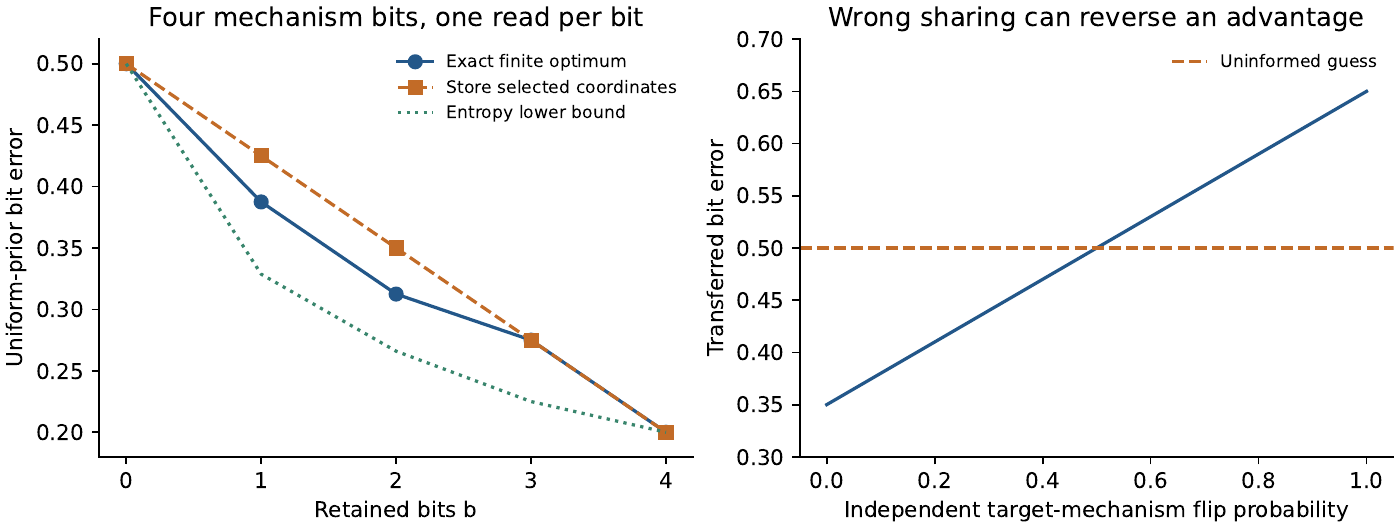
We enumerate every codebook of size exactly on for and . Restricting to exactly this size loses no optimum because adding codewords cannot worsen distortion. The total is codebooks. Distortion is an integer sum of Hamming distances divided by . The script independently evaluates each selected optimal encoder by summing over the original mechanism and observation , with exact rational channel probabilities at . Those original-model risks agree with (6) in all fourteen dimension/capacity cases.
| Codebooks, | Optimal risk, | Selected-coordinate risk | ||
|---|---|---|---|---|
| 0 | 16 | |||
| 1 | 120 | |||
| 2 | 1,820 | |||
| 3 | 12,870 | |||
| 4 | 1 |
The upper bound from selected-coordinate storage is not always sharp, but the gains do not persist at every capacity. At it equals the exact optimum. A sample of the risk frontier appears in Figure 1; the entropy converse is below the finite optimum at interior capacities. Neither the finite results nor that lower bound constitute a solved all-dimensional quantizer-design problem.
The script code/verify_and_plot.py writes the codebooks,
exact distortions, risks, and number of tied optimum codebooks to
data/finite_frontier.csv. It also records the maximum
conditional risk of the selected encoder over fixed mechanisms. That
last column is deliberately not called the minimax risk: the
search minimizes the average loss, and its deterministic tie-breaking
need not equalize errors. For instance, a zero-bit constant decoder has
Bayes risk
but error one on its complementary mechanism. A fair randomized
prediction improves that worst case, but a random-bit interface is
outside the deterministic code used in the enumeration.
All calculations use integers and fractions.Fraction.
The plots use floating-point conversion of those results. There is no
random seed because no Monte Carlo sample is drawn. Running the script
reproduces both the CSV files and the PDF/SVG artwork. Exhaustive
checking is limited to
and is not evidence about biological or learned architectures.
6 Sampling, shared mechanisms, and transfer
The main theorem fixes the observation budget at . To expose a separate sampling dimension, suppose there are independent repeated readings of each bit, with odd , and enough terminal memory to retain every coordinate majority (). Then each coordinate has error (9)
Proposition 6.1 (Sampling at full terminal capacity). For odd and , coordinate majorities are Bayes-optimal and their uniform-coordinate risk is . This risk is attained for every fixed mechanism. The complete vector is correct with probability . For , .
Proof. The prior factors and the observations are conditionally independent across coordinates. At a coordinate with observed ones, the posterior odds for one versus zero are when . Odd removes ties, so the unique MAP is majority. Its error is the binomial tail in (9), invariant under complementing the true bit. The errors of different coordinates are independent conditional on the mechanism, giving the displayed vector probability. The noiseless case follows directly. Substitution at gives . ◻
This is an elementary repeated-channel calculation already closely related to the finite-audit baseline. We do not present it as a second independent discovery. In particular, replacing by in Theorem 3.1 is exact only if the interface exposes solely those majority bits. With full repeated observations and , the encoder can use their different posterior reliabilities; discarding the counts first may be suboptimal. The following bounded exact computation demonstrates the loss; the general high-dimensional weighted quantization frontier remains unresolved. Section 8 below solves a two-coordinate extension.
Example 6.2 (Raw repeated readings outperform majority-only preprocessing). Take , readings per coordinate, , and , with the same uniform prior and late-query loss. If only the two coordinate-majority bits reach the encoder, the optimum is
since . With the full six-bit block, exact enumeration instead gives optimum , an improvement of . One attaining codebook is : retain one if the six readings contain more than three ones, otherwise zero, and use the retained bit as the answer to either coordinate query.For reproducibility without enumerating encoder maps, let count the ones at coordinate , and set when and otherwise. The exact joint probability is
For any decoder codebook , optimize the encoder separately at each count pair by evaluating (10) Counts retain the complete posterior because permutations within a coordinate block do not change its likelihood. There are four singleton codebooks and six pairs. Exact rational evaluation gives for every singleton, for the four adjacent pairs, and for the two opposite pairs. This exhausts all deterministic decoders; conditional linear minimization again excludes any improvement by randomization. The separate scriptcode/repeated_block_counterexample.py evaluates these ten
codebooks over sixteen count pairs and checks the concrete encoder
above. This original finite computation is retained as evidence;
Section 8 now supplies an analytic
two-coordinate extension, without an all-dimensional
repeated-observation theorem. It was added after independent review
identified this informative parameter case, then verified by a separate
count-based implementation.
If the same controls contexts and offsets are known, the retained estimate serves every context at the same risk. Its calibration budget is , independent of . A deliberately nonsharing controller forced to erase its estimate before entering each context needs observations to repeat this same calibration protocol. This comparison does not show an advantage over an unrestricted learner: any equally informed learner is allowed to retain and reuse the same statistic. The restriction, not architectural terminology, creates the separation.
Proposition 6.3 (Failure of an incorrect sharing assumption). Suppose target-context mechanism bits are , where the are independent of calibration and , with common flip probability . Transferring a decoder of source risk without adapting it gives (11)
Proof. For each coordinate, a target error occurs when the source estimate was wrong and no flip occurs, or when it was right and a flip occurs. Independence gives . Averaging over proves (11). ◻
For the one-bit three-coordinate code, and the target error is . At the old model has no predictive value; at its error is , worse than an uninformed guess. These are errors of the stipulated unadapted transfer rule. If were known, an equally informed controller would invert its predictions and recover the original error. Thus the counterexample concerns false or unrecognized invariance, not a failure of optimal Bayesian transfer under a correctly supplied target model.
7 Code, precision, and all-time memory are different resources
The retained register has at most states; its entropy need not equal , and a real-valued parametrization with one coordinate can still encode arbitrarily many distinctions if unlimited precision is silently granted. All states and codewords here are finite bit strings. A task-informed readout table also carries information even when it is immutable.
A direct full-table implementation uses at most bits for the encoder map and bits for the reconstruction vectors, before headers, offset tables, address logic, or working registers. This is an explicit upper encoding size, not a lower bound on the shortest program. A nearest-codeword implementation instead stores codeword bits and performs at most bit comparisons per encoding, with additional counting and loop workspace. Both can be described without self-model terminology. Neither cost is charged in (6).
The three-bit example is particularly transparent: a majority operation replaces the observed block by one retained bit, and a decoder replicates that bit. The encoder needs access to the observations while computing majority. It does not follow that a machine can process an arbitrary observation stream with one state bit throughout. The finite-audit baseline explicitly distinguishes peak decision-state widths from terminal output capacity; the present note preserves that distinction.
Even codebook optimization has a cost. The exhaustive search in Section 5 is a design-time calculation with exponential candidate counts. It is not a claim that the agent learns the optimal encoder from a small sample. All controllers in the theorem receive the specified statistical family and are permitted optimal design in advance. Learning an unknown factorization, pricing the search, or requiring a streaming encoder changes the frontier.
One can define a fuller research object (12) for peak and terminal memory, sample budget, operation budget , and immutable-code length in a specified machine model. For unrestricted machine models this display remains a proposal. Sections 9–10 solve sharply delimited streaming and literal-table versions. In particular, no universal statement follows by counting only retained parameter bits while ignoring an exponentially large decoder.
8 A sharp joint sampling result with one terminal bit
Here sampling is a decision variable, unlike the fixed calibration block in Theorem 3.1. Keep , a uniform independent prior and a late uniform coordinate query. At each of exactly steps, select either port and receive a fresh independent BSC() reading of that port, where is the same at both ports. The selection can depend on the complete preceding transcript. The offline encoder retains at most one bit; neither transcript nor action history survives separately. There is no peak-memory constraint in this subsection. Extend the earlier odd-sample definition to
Thus . A fixed deterministic tie decision has this Bayes error because the prior is fair; no random bit is needed to attain it.Theorem 8.1 (Two coordinates, one retained bit, adaptive sampling). Under this contract the optimum is Every fixed allocation of the readings between the two ports attains this value by retaining their overall majority and reconstructing or . Allocating all readings to one port and predicting only that coordinate also attains it. Adaptive allocation cannot improve it.
Proof. A deterministic one-bit decoder has at most two reconstruction words. A singleton gives error . Two different words are adjacent or opposite vertices of the binary square. For adjacent words, one coordinate is fixed, contributing to the total loss. The other coordinate must be estimated. Any adaptive experiment can be simulated from direct BSC readings of that coordinate: draw an independent fair nuisance bit for the other port, generate its noise internally, and consume the next unused direct reading each time the target port is selected. At most such readings are used. This randomized simulation has exactly the original joint law, so its binary estimation error cannot be below the Bayes optimum using all direct readings. This gives the stated lower bound.
For opposite reconstruction words , condition on , an event of probability . Write there. After subtracting from the reading at the selected port , the observation is through BSC(). Even with adaptive port choices, these are independent channel uses conditional on ; the actions supply no further information beyond the observations and independent seeds. Conditional error is at least . On the other two mechanisms either reconstruction has Hamming loss . Averaging gives again. Frozen independent seeds reduce randomized strategies to deterministic ones, without altering the fixed sample cap.
For any fixed allocation use and output the overall majority. When or , all readings measure the same bit and the conditional Bayes error is . For or the loss is always . Alternatively, all samples at one port give estimation error there and error on the unobserved coordinate. Both attain the bound. ◻
This proof also covers a hard upper bound of probes by padding a policy with ignored readings. It does not cover an expected sample cap, variable noise qualities, an early query, a nonuniform query, or a side channel revealing the final transcript. At , , so the formula gives . Example 6.2 now has an analytic extension; its original bounded enumeration remains independent evidence. The result also narrows the interpretation of that example: preserving reliability beats majority preprocessing, but balanced sensing does not beat concentrating all six probes at one coordinate under this Bayes loss.
Proposition 8.2 (Reliability formula for fixed independent observations). Let for independent coordinate experiments, and assume each has a distribution invariant under sign reversal. With one terminal bit and unrestricted encoding, For identically distributed nonzero posterior means, discarding magnitudes and retaining only signs before compression increases risk by .
Proof. Write a reconstruction as a sign vector . Its posterior loss is . An opposite pair optimizes to . Conditional on the magnitudes, sign symmetry and independence give , also when a magnitude is zero. An adjacent pair gives because the fixed bit’s mean is zero, and is therefore no better. A singleton gives . For iid nonzero means, each sign alone has constant reliability ; use for the difference. ◻
For odd repeated BSC readings and , posterior reliability is nonconstant and nonzero, so the gain is strictly positive. Even-sample ties need an explicit preprocessing convention and are not covered by the last sign-only statement. The general conditional-distortion reduction is standard remote coding; these low-dimensional consequences are proved here without a historical-priority claim.
9 Sharp separations under persistent streaming memory
A different machine reads a prescribed binary stream once in order, with state updated as . Its initial state is fixed. Only the state persists between reads. The external stage number is supplied, so tables may depend on ; code, clock, input wire and lookup hardware are distinct resources. There is no rereadable log. At completion the state is mapped to one terminal bit. “Width” means the largest number of persistent states at a layer, not total physical hardware memory.
For a Boolean encoder , two length- prefixes are equivalent if they induce the same function of the remaining suffix. Their number is the exact minimum number of reachable states at that layer in a deterministic ordered branching program. Necessity follows because merged states have identical future behavior. Sufficiency follows by storing the residual function and updating it by restriction to the arriving bit. This elementary standard construction is used here as an exact finite certificate. The same restriction-and-merging principle underlies reduced ordered Boolean decision diagrams [6, Theorem 1 and its proof]. The resource counted here is the maximum number of simultaneously reachable states in a fully layered encoder under the prescribed input order, not the total node count of a reduced diagram that may skip tests.
Theorem 9.1 (One-bit streaming penalty for three one-read coordinates). For , stream order , one terminal bit, and width at most two at every layer, the optimal Bayes risk is Width three attains the offline optimum . For , three persistent states are necessary to attain that offline optimum.
Proof. The posterior identity in Theorem 3.1 holds for every encoder, including streaming encoders, so minimize Hamming distortion. Codeword pairs at Hamming separation one or two have unrestricted distortion : the unchanged coordinates contribute each, and on two differing fair bits the average minimum distance is . Singletons give . An opposite pair attains only with its unique nearest-word rule, majority after fixed coordinate complementation. After two inputs, majority has three distinct residuals , the final bit, and . Width two cannot implement it. Distortion has denominator , so its next possible value is at least . The encoder uses width two and reconstructs or . It disagrees with majority only at , raising the total Hamming sum from six to seven. Width three implements majority through the three residuals, proving sharpness. ◻
At the streaming optimum is , a gap of above . This is a rigorous peak-state versus terminal-state separation, without any claim that the machine models human cognition or that the elementary branching-program argument is historically new.
Proposition 9.2 (Tie-aware three-state encoder for the six-read example). For the fixed blocked stream with three readings of each of two coordinates, and one terminal bit, exactly three peak persistent states are necessary and sufficient to attain .
Proof. Opposite words are strictly better than adjacent ones here by Proposition 8.2; each coordinate’s three-read reliability has two distinct magnitudes with positive probability. For the posterior-optimal output is forced to be the overall majority whenever the six-bit total differs from three. Ties have zero excess conditional loss. Let be the number of ones in the first three readings and let be the last three. Choose the tie rule
It has the required sign at every nontie. Its residual-state counts after inputs are . At layer three the residuals are , , and ; at layer four they are ; at layer five they are . At layers one and two the first-block count yields at most two and three classes. Thus the residual construction gives width three. Notice that storing the literal first-block count would use four states; the residual construction merges the loss-equivalent counts zero and one at layer three.For necessity, restrict the six input bits to . Totals are even, so none is a tie, and the output is forced to be majority of . Composing each pair of transitions would implement majority of three using the same width; Theorem 9.1’s residual argument forbids width two. For the other opposite codebook complement the appropriate coordinate block first and apply the same argument. Every raw input has positive probability in the stated parameter range, so nontie mistakes strictly increase risk. ◻
A strict “total exceeds three” tie rule needs four states. Optimal-risk state complexity therefore requires optimizing loss-neutral ties, not merely minimizing the machine for an arbitrarily chosen optimal offline encoder. The exact residual certificates and all truth tables are in the new review and verification files. Three states require two physical binary state bits if implemented by a conventional register; the terminal output needs one.
10 An exact finite design problem with explicit code and lookup charges
The broad frontier in Section 7 remains unsolved for general machines. The following restricted model makes one version fully finite. Joint design through deterministic information states has substantial precedent, including Mahajan and Teneketzis [11, Sections 4–5]; continuous memory-control formulations such as Tottori and Kobayashi [14] do not supply finite-bit bounds. Finite-time finite-memory testing also predates this note [7]. We use those methodological distinctions rather than claiming a new dynamic-programming principle.
Fix an integer horizon , positive integer state counts , and an integer terminal symbols. At stage , the controller uses tables
The selected port yields a fresh BSC observation. Finally use and a binary reconstruction table . The late query reveals no additional hidden-state information. All tables are chosen before the mechanism. A supplied external clock addresses the stage. There is no physical posterior register and no persistent scratch.Proposition 10.1 (Designer joint-mass recursion). Let and . For a selected whole pair of tables , define At the terminal layer put The backward recursion and returns the exact Bayes optimum over this finite table class. For rational it can be evaluated by finite exact arithmetic on reachable joint masses.
Proof. The displayed update is the law of total probability for an admissible state-based controller. Terminal coordinatewise Bayes decisions give . Every feasible controller is a sequence of whole tables and conversely every such sequence is feasible. Induction over the finite horizon therefore proves the recursion. Different paths with the same joint mass have the same feasible continuations and terminal costs. Crucially the minimization selects one whole map, not separate actions for latent or histories already merged into the same state. The joint mass is a designer’s object; the online controller executes only the chosen tables. ◻
Literal code and operations.
With dimensions and alphabet conventions supplied to both sides, a padded fixed-width serialization of these tables has exactly
bits. Invalid binary indices are disallowed. Initial state is fixed. Headers, clock, address logic, sensor and input wire are outside . In a unit table lookup model execution uses lookups: one action and one transition per sample, one final compression, and one query-specific output lookup. Sampling uses calls. This is an exact accounting convention, not a universal bit operation, latency, energy or shortest-program lower bound. Special-purpose Boolean circuits and compressed tables belong to different contracts.For prescribed caps on sample count, persistent width, literal table bits and lookup count, enumerate finite satisfying those caps and apply the recursion. This exactly solves that bounded literal-table design problem in principle, although design complexity is enormous. With a supplied clock, state counts measure layer-boundary storage. If the clock must be internal, a direct homogeneous implementation stores and uses at most states before terminal erasure; no optimal clock-storage bound is asserted. State-dependent resource counters must themselves be stored if they affect future decisions.
The policy class here is deterministic. For fixed alphabets, horizon and full-table resource charges, allowing independent random choices cannot improve Bayes loss: fixing all choices yields an admissible deterministic table sequence. This argument does not preserve arbitrary expected resource budgets or arbitrary compressed program lengths. For example, with one fair bit and an optional noiseless read of cost one, an expected budget allows a random read with probability , attaining error ; a deterministic initial decision obeying that expected cap cannot read and has error .
Concrete code witnesses.
For the blocked six-read example, residual automata for the optimized tie rule, strict threshold, and majority of the first five readings have literal lengths 73, 83, and 69 bits respectively, under the serialization above. All use six sample calls, 14 lookups, and have risk at . Their peak state counts are three, four, and four, while all three use two binary state bits. Thus fewer reachable states need not mean the smallest literal table, even among these three equally accurate encoders. These are verified implementation witnesses, not globally shortest programs. The last machine consumes and ignores its sixth reading to preserve the fixed-horizon contract. The code generates explicit tables, their exact bitstrings (with headers external), and checks every input against its defining function.
Exact new computations.
The new resource_frontier.py exhausts reachable joint
masses for width two, canonicalizing only the exchange of state labels.
At
,
,
adaptive port choices and
give respectively
Separately, 180 exact codebook searches cover all allocations of probes to two coordinates at and agree with Theorem 8.1. These are finite consistency checks; the adaptive all- conclusion rests on the proof, not on enumeration.
11 Unequal channels, higher dimension, and an executable adaptive gain
This section strengthens the resource examples while narrowing their novelty interpretation. Classical random access coding already contains the uniform late-coordinate task: Ambainis et al. [1, Section 2.3, Theorem 2 and Eq. (25)] prove one-bit majority coding optimal, and Kondo et al. [9, Section III-A, Eqs. (23)–(24) and (49)] give exactly the cube-codebook objective for the noiseless average criterion. Thus neither the majority example nor finite codebook optimization is a new coding principle. Conditional distortion supplies the noisy specialization. Weighted posterior scores also overlap biased random access coding [12, Section II, Lemma 1; Section IV.1]. The additions below are self-contained specializations, finite separation certificates, and implementations; historical priority remains unverified.
11.1 Two coordinates: unequal noise still need not reward adaptation
Proposition 11.1 (Unequal-channel extension). In Theorem 8.1, allow known port-specific crossover probabilities , with fresh independent noise. Put . The optimal one-terminal-bit risk is Observing only a best port attains it. Adaptive allocation cannot improve it; in contrast to the equal-channel theorem, arbitrary fixed allocations need not attain it.
Proof. If , a BSC() sample is a BSC() sample followed by an independent flip with probability . For an opposite reconstruction pair, conditional on the matching mechanisms, the entire adaptive transcript is therefore a simulation from best-channel readings of the common bit. Its error is at least ; on the other mechanisms the loss is . For an adjacent pair, the fixed coordinate contributes , and target-coordinate observations can likewise be simulated from best-channel readings, with independent nuisance bits and noise for the other port. The proof of Theorem 8.1 gives the lower bound. Repeatedly observe a best port to attain it. At all readings are uninformative and both sides are ; is covered by the same simulation, including the case. ◻
This is the standard channel-simulation technique also used in D02’s binary experimental-design note, applied to a different terminal coding loss. It is a negative result for adaptive advantage, not an independent discovery of the technique.
11.2 One terminal bit in arbitrary dimension
Proposition 11.2 (Fixed product experiments; posterior-score form). Let fair independent mechanism bits undergo fixed independent coordinate experiments. Suppose has a sign-symmetric distribution for every . Then the optimal one-terminal-bit risk is A full opposite pair of reconstruction words attains it. The experiments need not have equal accuracy or equal sample counts.
Proof. Use sign-valued reconstructions and let be the set where they differ. Optimizing the encoder chooses the larger posterior score,
The first term has expectation zero. Independence and individual sign symmetry remove the signs in the second. Adding an omitted independent mean-zero cannot decrease the expected absolute value, by conditional Jensen. Thus is optimal. A singleton is no better. Posterior Hamming loss is minus score divided by , giving the formula. ◻For one BSC read per coordinate this is weighted majority with . In the equal-noise case it recovers the classical one-bit random-access formula
whose noiseless case is already explicit in Ambainis et al. [1]. Random posterior reliabilities after repeated readings retain the same conditional-distortion interpretation. This proposition’s independent unconditional posterior-mean assumption must not be silently applied after adaptive sampling.11.3 Adaptive acquisition: a separate reduction and a finite separation
For fresh independent port-specific BSC observations, full acquisition workspace, exactly probes, and one terminal bit, it still suffices to optimize a full opposite decoder pair. This assertion uses a different argument. Any decoder pair differs on a subset ; its fixed coordinates contribute unconditionally. Observations outside can be simulated by independent nuisance bits and noises. Replace their physical probes by ignored probes in to preserve the hard sample count. Freeze the simulation’s independent seed at a value with no worse Bayes loss. Complement coordinates in as needed to standardize the decoder pair. The resulting policy probes only , and a full opposite pair under that policy has the same risk, because the untouched actual coordinates have posterior mean zero and contribute each. A singleton gives and can be handled separately. This reduction uses unrestricted workspace and is not itself a streaming-memory construction.
For , let be observed ones minus zeros at port , and put
The known adaptive actions introduce no extra likelihood factor after the transcript is conditioned upon. Its posterior still factors by coordinate. With probes left, define the design recursion The optimal full-history Bayes risk is . This is ordinary finite-horizon Bayesian experimental design, not a new general recursion. The posterior vector is only a designer’s calculation. The actual witnesses below are compiled to finite state tables.Proposition 11.3 (A verified three-coordinate adaptive separation). For , , , and one terminal bit, an adaptive policy attains . Every fixed allocation has risk at least , even with optimal offline encoding and decoding. The gap is .
Proof. Read each port once. If all three readings agree, preserve their common bit and consume two ignored readings. Otherwise choose the lowest-index port carrying the majority sign and read it again. If that fourth reading agrees with the majority, the answer is committed: consume an ignored fifth read at any fixed legal port (mathematical port 1, represented by index 0 in the C implementation). If it disagrees, read the selected port once more and use that final bit. This has the same decision as an experiment that takes two further readings at the selected port: when its first two readings agree, the third cannot change their majority, so replacing that last reading by any ignored probe preserves the decision and its loss. Decode the retained bit identically at all three coordinates.
Write . The first three readings are independent fair bits. On the all-equal event, of probability , the retained original sign has expected posterior score . On the mixed event, the other two single-read means cancel. In the equivalent three-read experiment just described, the expected absolute posterior mean of the selected port is . Conditioning on the first reading’s sign does not change this expected magnitude, by bit-flip symmetry. Thus this policy’s risk is
At , this is .For fixed sampling, permutation symmetry leaves the five count partitions in the following table. Each is evaluated with optimal decoding by Proposition 11.2, not by imposing the adaptive policy’s decoder. For a port with readings and ones, its mass is and its posterior mean is the likelihood difference divided by that likelihood sum. Substituting these finite rational masses into the displayed proposition gives
These exhaust fixed allocations, and random mixtures of fixed allocations cannot beat their minimum. Exact independent original-model enumeration checks every decoder pair for all allocations, reproducing the table. ◻The same exact dynamic program gives global adaptive optimum ; a separate implementation checks all 28 decoder pairs against the original latent likelihoods, without assuming the opposite-pair reduction. This finite optimality computation is distinguished from the explicit policy proof of a strict adaptive-versus-fixed separation.
Unequal channels also admit a positive three-coordinate example. Take four probes and crossover probabilities , , and . Exact computation gives adaptive risk and fixed-allocation optimum , a gap of . The attaining fixed allocation is ; both optima are independently checked over all 28 decoder pairs. A full table specifies the adaptive policy in the artifact. Larger bounded exploration includes , with computed gain . These finite values do not establish a general scaling law or an all-dimensional adaptive formula. Zero-gain cases are also retained in the data.
11.4 Executable witnesses and actual storage accounting
Adaptive states must determine future actions as well as answers. Merging prefixes merely because they have the same final Boolean output function can incorrectly erase which sensor must be read next. We construct residual trees labeled by the next port and both observation continuations. The equal-noise adaptive witness has layer widths ; a best fixed-allocation witness has . These are implementation upper bounds, not minimum-width claims over all optimal policies.
The C99 implementation tags each state by its layer, making the clock
part of the persistent state. It uses one caller-owned
uint8_t state, no retained history or heap, and a read-only
array of four-byte nodes: next port, zero successor, one successor, and
output. Terminal nodes loop and retain the terminal bit. The current
sensor input and ordinary CPU/ABI working storage remain outside the one
persistent byte. After completion only two terminal tags are possible,
so the retained data alphabet has one bit of capacity. The physical C
byte does not shrink; its fixed terminal-stage information carries no
additional information about the mechanism.
| Witness | Probes | Error | Tagged states | Table bytes | Literal bits |
|---|---|---|---|---|---|
| Equal, adaptive | 5 | 19 | 76 | 108 | |
| Equal, best fixed | 5 | 13 | 52 | 60 | |
| Unequal, adaptive | 4 | 13 | 52 | 64 | |
| Unequal, best fixed | 4 | 12 | 48 | 60 |
The equal adaptive/fixed tagged states require five/four logical bits; the unequal pair requires four/four. Byte allocation rounds all four to one. The unequal example therefore fits a common cap of one persistent byte and 52 read-only table bytes, with both controllers using four probes. Its gain is not obtained by giving the adaptive controller an uncharged history. The fixed comparator is already optimal even with unlimited encoding workspace; it is not deliberately memory-handicapped. Different code and state Pareto optima remain open.
On the recorded x86-64 GCC 14.2.0 build with -O2, all
four object files have 102 bytes of .text for the five
small exported functions, including the table-size inspection function;
their .rodata sizes are exactly those in Table 3. Compiler stack-use reports
charge eight bytes per function. Object metadata, dynamic-loader
footprint, caller/test-harness storage, registers, sensor electronics,
and instruction latency or energy are not represented by the one-byte
persistent-state claim. This is executable synthetic validation, not a
measurement of a physical agent. The source is portable C99; these ABI
measurements are specific to the recorded build. We make no
shortest-program or minimum-hardware claim.
For probes, the C interpreter performs action reads, transition reads and one output read: table accesses. Its function calls also include initialization. The earlier literal model counts a separate terminal compression lookup and hence lookups; the C implementation fuses that trivial step. Both conventions are exposed instead of silently comparing their operation counts.
Every generated binary was executed on every raw response sequence (32 or 16 per policy), including its actual adaptive port selections. The resulting outputs were evaluated by exact summation over all eight hidden mechanisms with the original port-specific channel probabilities. A separate reviewer compiled and tested all four sources independently. New verification also covers 63 two-coordinate channel cases, including unequal noise, 1,140 higher-dimensional codebooks, and 21 acquisition-frontier rows. Independent reviewer implementations add 60 unequal-channel cases including noiseless and uninformative endpoints, and all-pair adaptive and fixed-allocation checks. No Monte Carlo estimates are used for these finite certificates.
Readiness has improved through explicit claims and executable evidence, but novelty evidence has become more conservative: the newly documented random access-code antecedents subsume more of the original baseline than v2’s source audit identified. Related late-query streaming problems already have substantial lower-bound literature [5, Theorem 2]; their target is the majority of empirical streams, whereas ours is the hidden mechanism bit, so those bounds cannot simply be transferred. Historical priority of the finite adaptive examples, robustness beyond the supplied model, and human specialist assessment remain unresolved.
12 Interpretation, distinctness, and publication readiness
Being.
The current retained statistic supports a precise prediction capability: the attainable Bayes risk in (6). This is a task-relative account of available information, not a measure of the system’s existence or consciousness.
Becoming.
Calibration changes the evidence, compression changes the distinctions retained, and transfer changes where that evidence is used. Better organization can lower average risk without increasing the number of retained bits. It can also discard distinctions that a later task needs; no monotonic developmental conclusion follows.
The MIND.
A mechanism model can be a reusable representation of how the agent’s commands produce outcomes. The model is functionally self-relevant because its parameter belongs to the stipulated actuator. The same information can be represented by a codeword index or compiled controller state. Efficiency and reuse are operational claims. They do not establish subjective introspection or a privileged conscious architecture.
D06 asks whether a prescribed family of old capabilities survives a fixed replacement, uniformly over states, with possible side records and future actions. This note instead optimizes average risk after noisy acquisition under a terminal bit budget. The two share coding ideas but have different quantifiers, objectives, and acquisition assumptions. Their basic pigeonhole arguments should be cross-referenced, not counted twice as novelty. No mandatory merge of the two mathematical drafts is recommended. For publication, however, this note is better treated as a resource continuation of the existing reflective-model/audit line with the new finite streaming and sampling results offered as explicit additions. Their historical novelty remains unverified.
Unresolved research proposals.
The strongest next target is a scalable joint memory–sample–computation frontier beyond the finite three- and four-coordinate cases in Section 11, with strict streaming and executable code constraints. The exact finite table recursion is a specification and small-instance solver, not an efficient general synthesis algorithm. Another is transfer when the shared mechanism must itself be inferred rather than supplied. A third is a robust resource frontier when a bounded fraction of contexts violate invariance. The narrow results above do not solve these general questions. We do not label a plausible extension a theorem or invent a conjecture merely to make the note look more research-like.
Readiness.
This complete technical-note draft provides proofs, exact finite data, editable figures, source locators, and internal review records. Its main formula is established source-coding mathematics under a transparent operational interpretation. It is not a stand-alone claim of a newly discovered information law, and broad significance or priority requires further work and external expert assessment. Current targeted searches also identify nonasymptotic noisy source coding [10]; its excess-distortion criterion differs from our expected-loss identity. The revised manuscript and its exact computations underwent fresh specialist and hostile AI-agent review. These are internal AI reviews, never external human peer review.
References
- Andris Ambainis, Debbie Leung, Laura Mančinska, and Maris Ozols. Quantum random access codes with shared randomness, 2009. URL https://arxiv.org/abs/0810.2937v3. arXiv:0810.2937v3, 14 June 2009; first submitted 2008. Classical average-case Section 2.3 inspected.
- B-Theory. Finite noisy audits with learned baselines: Exact risk, interface-dependent memory, and a matched compiled controller, 2026. URL https://www.b-theory.com/manuscripts-html/finite-noisy-audits/. Technical addendum v1.0, 9 November 2026; source assigns no individual author line. Accessed 13 November 2026.
- B-Theory. When does an explicit self-model help? calibration and control under internal change in a finite-state pilot, 2026. URL https://www.b-theory.com/manuscripts-html/reflective-self-models/. Final R4 working manuscript, 14 October 2026; reading copy prepared 16 October. Source supplies no named individual author. Accessed 13 November 2026.
- Tomer Berg, Or Ordentlich, and Ofer Shayevitz. Binary hypothesis testing with deterministic finite-memory decision rules, 2020. URL https://arxiv.org/abs/2005.07445v1. arXiv:2005.07445v1, 15 May 2020; inspected six-page preprint, distinct from the conference record.
- Mark Braverman, Sumegha Garg, and David P. Woodruff. The coin problem with applications to data streams. In Proceedings of the IEEE Symposium on Foundations of Computer Science, 2020. URL https://www.cs.cmu.edu/afs/cs/user/dwoodruf/www/bgw20.pdf. Theorem 2 concerns empirical-majority late queries, not the present hidden-bit loss.
- Randal E. Bryant. Graph-based algorithms for Boolean function manipulation. IEEE Transactions on Computers, C-35(8):677–691, 1986. doi: 10.1109/TC.1986.1676819. URL https://www.cs.cmu.edu/~bryant/pubdir/ieeetc86.pdf.
- Richard A. Flower and Martin E. Hellman. Hypothesis testing with finite memory in finite time. IEEE Transactions on Information Theory, 18(3):429–431, 1972. URL https://www-ee.stanford.edu/~hellman/publications/10.pdf.
- Alon Kipnis, Stefano Rini, and Andrea J. Goldsmith. Indirect rate-distortion function of a binary i.i.d source, 2015. URL https://arxiv.org/abs/1505.04875v2. arXiv:1505.04875v2, 4 June 2015; the inspected 9-page preprint edition.
- Ruho Kondo, Yuki Sato, Hiroshi Yano, Yota Maeda, Kosuke Ito, and Naoki Yamamoto. Random access codes: Explicit constructions, optimality, and classical–quantum gaps, 2026. URL https://arxiv.org/abs/2604.21274v3. arXiv:2604.21274v3, 16 July 2026; Section III-A inspected.
- Victoria Kostina and Sergio Verdú. Nonasymptotic noisy lossy source coding, 2016. URL https://arxiv.org/abs/1401.5125v2. arXiv:1401.5125v2, 16 September 2016; introduction and criterion inspected.
- Aditya Mahajan and Demosthenis Teneketzis. A decision theoretic framework for real-time communication, 2005. URL https://arxiv.org/abs/cs/0511026. arXiv:cs/0511026v1, 6 November 2005; Sections 4–5 inspected.
- Gabriel Pereira Alves, Nicolas Gigena, and Jędrzej Kaniewski. Biased random access codes. Physical Review A, 108:042608, 2023. URL https://arxiv.org/abs/2302.08494v3. arXiv:2302.08494v3; fixed-decoder score and weighted-majority comparison only.
- Mateo Rojas-Carulla, Bernhard Schölkopf, Richard Turner, and Jonas Peters. Invariant models for causal transfer learning. Journal of Machine Learning Research, 19(36):1–34, 2018. URL https://jmlr.org/papers/v19/16-432.html.
- Takehiro Tottori and Tetsuya J. Kobayashi. Memory-limited partially observable stochastic control and its mean-field control approach. Entropy, 24(11):1599, 2022. doi: 10.3390/e24111599. URL https://arxiv.org/abs/2203.10682.